Volatility Drag: Why Your Average Return Overstates Your Wealth
Volatility drag is the gap between an investment's average return and the rate it actually compounds at: roughly half the variance. Where it comes from and what to do about it.
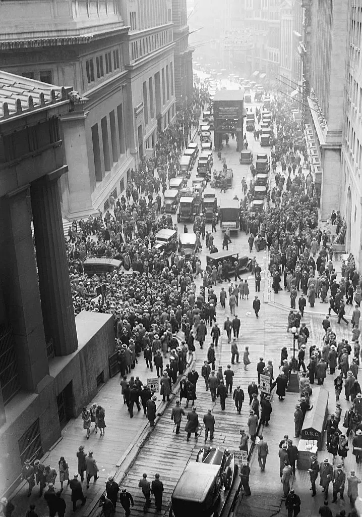
On the image The Dow lost 89% between its 1929 peak and its 1932 low. To get back it had to gain more than 800%, and in price terms it did not return to the 1929 high until 1954. A crowd fills Wall Street outside the New York Stock Exchange during the crash, 29 October 1929. Photo: United States government, public domain, via Wikimedia Commons.
Volatility drag is the gap between the average return of an investment and the rate at which it actually compounds. For returns that are not too large, the compound growth rate is roughly the average return minus half the variance, $G \approx \mu - \sigma^2/2$. The more an investment swings, the more its average return overstates what you end up with.
This is the short version of an argument I make at length in Finance Is Geometry. If you only read one thing about it, read this.
#A year that averages zero and loses money
Start with 100 dollars. It goes up 50%, then down 50%.
- After the gain: $\$100 \times 1.5 = \$150$
- After the loss: $\$150 \times 0.5 = \$75$
The average of the two returns is zero, and you lost a quarter of your money. The loss was applied to 150 dollars, the gain to 100 dollars, so the loss took away more than the gain added. Nothing exotic happened. This is what compounding does to anything that swings.
The same asymmetry shows up in the gain you need to recover from a loss:
| Loss | Gain needed to break even |
|---|---|
| 10% | 11.1% |
| 20% | 25% |
| 50% | 100% |
| 80% | 400% |
| 89% | 809% |
The last row is the Dow Jones Industrial Average from September 1929 to July 1932. In price terms it took until November 1954 to get back to its 1929 peak.

If recovery were symmetric it would track the dashed line. The deeper the loss, the further the required gain runs away from it.
#The formula
The general rule is that a loss of $L$ needs a gain of $L/(1-L)$ to recover. For a whole sequence of returns, the number that matters is the average of $\ln(1+R)$, the log of each period’s growth factor, because logs turn the multiplication of compounding into addition. Expanding that around the average return $\mu$ gives
$$G = \mathbb{E}[\ln(1+R)] \approx \mu - \frac{\sigma^2}{2}$$
where $\sigma^2$ is the variance of returns. In continuous-time finance the same term appears exactly: under geometric Brownian motion, log wealth drifts at $\mu - \sigma^2/2$, not at $\mu$.
Some numbers. A portfolio averaging 10% a year with 20% volatility compounds at roughly 8%. Two funds that both average 10% a year, one with 10% volatility and one with 30%, compound at roughly 9.5% and 5.5%. Over thirty years that is the difference between turning 10,000 dollars into about 150,000 dollars and into about 50,000 dollars. The average return is the same, and the ending wealth differs by a factor of three.
#Why it happens
The logarithm bends downward. Take the two outcomes from the example, a factor of 1.5 and a factor of 0.5, and mark them on the log curve. Averaging the factors first gives 1.0, and $\ln 1.0 = 0$. Taking logs first and then averaging gives $\frac{\ln 1.5 + \ln 0.5}{2} \approx -0.144$. The second is below the first because the straight line between two points of a downward-bending curve sits under the curve.

Averaging first lands on the curve at zero. Taking logs first lands on the chord, below it, at about −0.14. That vertical gap is the cost of variance.
That is Jensen’s inequality: for a concave function, the average of the function is at most the function of the average. Applied to wealth it says $\mathbb{E}[\ln(1+R)] \le \ln(1 + \mathbb{E}[R])$, with equality only when returns never vary. The $\sigma^2/2$ formula is the first term of the gap.
#Which average is yours
The arithmetic average is not wrong. It is the right number for one period, or for the average result across many investors who each hold the asset once. It is the wrong number for one investor holding it through many periods, which is what most of us do. That investor lives the compound rate.
The gap between those two averages is what makes wealth non-ergodic, which I explain with a single coin in Ergodicity, Explained.
Open this simulation in Explore →
Set the average return to 10% and move the volatility. At 0% every path is the red line. At 20% the median investor compounds near 8%, and at 40% near 2%, with the same average return throughout.
#What to do about it
If volatility is a cost, then reducing it is worth something even when it does not raise the average return.
Diversify. Combining assets that do not move together lowers $\sigma^2$ for a given $\mu$. The drag falls with the square of volatility, so halving volatility cuts the drag to a quarter.
Be careful with leverage. Doubling your exposure doubles $\mu$ and quadruples $\sigma^2$. Past a point, more leverage lowers the growth rate, and the point where growth is highest is the Kelly fraction, which in this approximation is $\mu/\sigma^2$ with $\mu$ measured above the risk-free rate.
Cut the worst losses. Because the drag comes from the size of the swings, the large losses do most of the damage. Paying a small, steady cost to remove them can raise the compound rate even though it lowers the average. That is the case for tail hedging, which I tested with seventeen years of options data in the tail hedge debate.
#What the data says
The formula is not just a model. Take the forty currencies in forex-centuries, the open dataset of exchange rates I assembled for Leptokurtic, with yearly data going back as far as 1791. For each one, measure the gap between the average yearly change in its exchange rate against the dollar and the compound yearly change, and compare it with what $\sigma^2/2$ predicts.
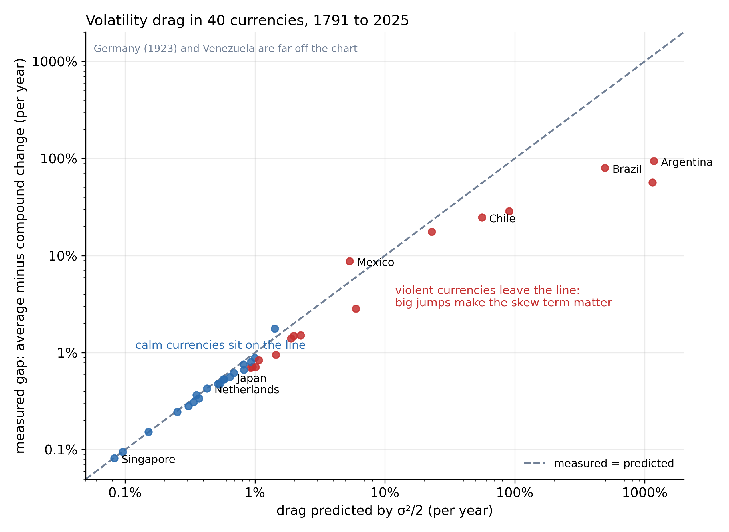
Each point is one currency. Blue points are within 25% of the prediction, red points are not.
For calm currencies the match is almost exact. The Netherlands shows a measured gap of 0.430% a year against a predicted 0.429%; Singapore, 0.082% against 0.083%. Past a few percent a year the points leave the line. $\sigma^2/2$ is only the second-order term, and the next one, $+\mathbb{E}[R^3]/3$, gets large when the moves are big and lopsided. Here the big moves are devaluations, jumps in the price of a dollar, which pull the measured gap below the prediction. For someone holding the peso or the real, the same jumps are losses, and they push the drag the other way.
#Checked in Lean
The formula is proved, not just derived, in lean-ergodicity. For any finite distribution of returns smaller than 100%, the compound growth rate equals $\mu - \sigma^2/2 - \mu^2/2$ up to an error the theorem bounds explicitly. The extra $\mu^2/2$ is the price of working in discrete time; it vanishes in the continuous-time version.
theorem volatility_drag (s : Finset ι) (w R : ι → ℝ)
    (hw : ∀ i ∈ s, 0 ≤ w i) (hsum : ∑ i ∈ s, w i = 1) (hR : ∀ i ∈ s, |R i| < 1) :
    |∑ i ∈ s, w i * log (1 + R i) -
        (mean s w R - variance s w R / 2 - mean s w R ^ 2 / 2)| ≤
∑ i ∈ s, w i * (|R i| ^ 3 / (1 - |R i|))#The limits
The $\sigma^2/2$ formula is an approximation for small, roughly normal returns. Real returns have fat tails, and the higher moments move the drag away from $\sigma^2/2$ in both directions: big losses (negative skew) make it worse, big gains (positive skew) make it smaller, and large kurtosis adds to it. The exact quantity is always $\mathbb{E}[\ln(1+R)]$, and when one loss is large enough to wipe you out, no formula based on variance captures it. Zero is a point you do not come back from.
#Further reading
- Finance Is Geometry, and It All Comes Back to Jensen’s Inequality: the long version, with the Taylor expansion, Itô’s lemma, Kelly and fat tails.
- Ergodicity, Explained: the same gap seen as time averages against ensemble averages.
- The Leptokurtic series: two thousand years of financial data, crash detection, and tail hedging on real options.
From the series One Path.
Written with an LLM in the loop, like everything here. The ideas and the mistakes are mine. More on how I write.