
Finance Is Geometry, and It All Comes Back to Jensen’s Inequality
Logarithms, Kelly, ergodicity, and tail risk meet at the same geometry: wealth compounds multiplicatively, the logarithm is concave, and Jensen's inequality measures the cost of variability.
On the image Each chamber is the previous one scaled by the same factor, so the shell grows by multiplication and traces a logarithmic spiral. Wealth compounds the same way, which is why the logarithm is the right ruler for it. A nautilus shell cut in half to show its chambers. Photo: Chris 73, CC BY-SA 3.0, via Wikimedia Commons.
Never cross a river that is on average four feet deep. If the river is eight feet deep in the middle and dry on the sides, the average tells you nothing about whether you will drown. You will drown in the middle, or you won’t. There is no averaging across parallel universes where you both survive and die.
The same asymmetry shows up wherever outcomes compound. Lose 50% of your wealth and you need a 100% gain just to break even, because the loss hits a larger base than the recovery builds from. Going from $100 to $200 and from $200 to $400 are different dollar amounts but the same proportional move: one doubling. Wealth is about ratios and scaling, not absolute differences.
This multiplicative structure has consequences that run deeper than intuition suggests. The mathematics that governs survival in compounding environments was invented 400 years ago to help astronomers multiply large numbers, partially rediscovered in the 18th century to solve a paradox about gambling, formalized again through information theory, and then largely obscured by theories that optimized across hypothetical worlds instead of along a single path through time.
That is the geometric claim in this essay: wealth evolves multiplicatively, while most ordinary intuition is additive. The logarithm is the change of coordinates that lets us move between those two descriptions.
This is the story of why geometry sits at the core of finance, why a single inequality ties the whole picture together, and why reducing variance can be more valuable than increasing returns.
None of the parts are mine. Kelly, Peters, Spitznagel, and Taleb each worked one of them out. My only claim is that they are the same picture, and this essay traces how the pieces fit.
#I. The Invention of Linearization (1614)
In the early 17th century, astronomers were drowning in calculation. Johannes Kepler had just published his laws of planetary motion, and navigators were trying to compute positions using spherical trigonometry. A single problem might require multiplying two seven-digit numbers, a process that took skilled calculators half an hour and was prone to error.
John Napier, a Scottish laird and amateur mathematician, spent 20 years searching for a way to simplify this. His insight: if you could convert multiplication into addition, calculations would become trivial. He invented “logarithms” (from Greek logos = ratio, arithmos = number), a table that mapped every number to its “ratio-representative.”
The crucial property: $\log(ab) = \log(a) + \log(b)$. Multiplication becomes addition. Division becomes subtraction. Exponentiation becomes multiplication.
But Napier’s invention was more than a computational trick. He had discovered the mathematical tool for linearizing multiplicative processes. Four hundred years later, this same tool would reveal why volatility destroys wealth and why tail hedging works.
#II. The Number That Grows Continuously (1680s)
In the 1680s, Jacob Bernoulli investigated a financial puzzle: if you lend money at 100% annual interest, what happens if you compound it more frequently?
- Annually: $(1 + 1)^1 = 2$
- Monthly: $(1 + 1/12)^{12} \approx 2.61$
- Daily: $(1 + 1/365)^{365} \approx 2.71$
Bernoulli showed that as the compounding interval shrinks toward zero, the result approaches a limit:
$$e = \lim_{n \to \infty} \left(1 + \frac{1}{n}\right)^n \approx 2.71828$$
The number later denoted by $e$ emerges naturally from continuous compound growth. It is the base of the logarithm that measures growth rates, the “natural” logarithm $\ln(x)$. Where Napier gave us the tool to linearize multiplication, Bernoulli identified the constant that emerges when growth becomes continuous.
Together, Napier and Bernoulli provided the mathematical foundation: wealth grows multiplicatively, and logarithms convert this multiplicative growth into additive increments.
#III. Jensen’s Breakthrough (1906)
The missing geometric step arrived in 1906. Danish mathematician Johan Jensen proved the inequality that now bears his name. He showed that whenever a function is concave, averaging inputs before applying the function gives a larger result than applying the function first and then averaging.
That result sounds abstract, but it is exactly the bridge this story needs. Napier gave us logarithms. Bernoulli showed why the natural logarithm belongs to compounding. Jensen explained why variability hurts once the relevant function bends downward.
#IV. Jensen’s Inequality: The Geometry of Concavity
A function is concave if it bends downward. If you draw a straight line between two points on the curve, that line sits below the curve itself. The logarithm is concave. That simple geometric fact turns out to matter enormously in finance, because wealth compounds.
There is a reason the logarithm is the right function here, not just a convenient one: it is the map that turns multiplicative wealth dynamics into additive increments you can sum through time. In raw wealth space, returns multiply. In log space, they add. Jensen’s inequality matters because this change of coordinates is not linear: the map bends downward, and that bend is exactly why dispersion in returns becomes a drag on long-run growth.
Jensen’s Inequality states that for a concave function $\varphi$:
$$\mathbb{E}[\varphi(X)] \leq \varphi(\mathbb{E}[X])$$
The notation is simple once you unpack it. $\mathbb{E}[X]$ means the expected value, or average, of $X$. The symbol $\varphi(X)$ means “evaluate the function $\varphi$ at $X$.” So the inequality says: for a concave function, the expected value of the transformed variable is less than or equal to the transformed expected value. The gap between those two quantities is the Jensen gap. It is the mathematical penalty created by variability under concavity.
Here is the simplest possible example. Suppose your wealth factor is either $1.5$ or $0.5$ with equal probability. In other words, you either gain 50% or lose 50%.
- The arithmetic average wealth factor is $(1.5 + 0.5)/2 = 1.0$
- The log of that average is $\ln(1.0) = 0$
- But the average log is $\frac{\ln(1.5) + \ln(0.5)}{2} \approx -0.144$
So the average outcome looks flat, but the expected log-growth is negative. Under repeated exposure to the same kind of multiplicative gamble, that means long-run compound growth is negative even though the arithmetic average looks harmless. That is Jensen’s inequality in action.
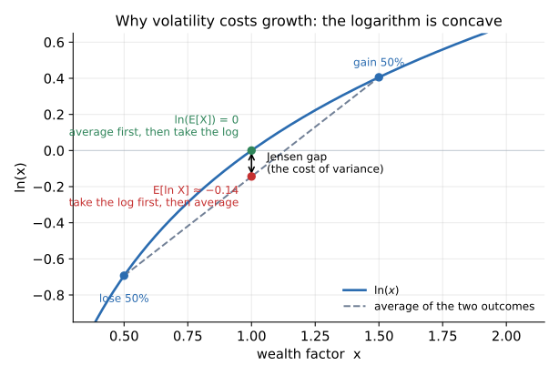
The whole effect in one picture. Mark the two outcomes on the curve, ×0.5 and ×1.5, and draw the straight line between them. Averaging first and then taking the log lands on the curve at $\ln(1.0)=0$ (green). Taking the log first and then averaging lands on the chord, below it, at about $-0.14$ (red). Because the logarithm bends down, the second is always lower. That vertical gap is the cost of variance.
To see this more viscerally, start with $100:
- After a 50% gain: $$100 \times 1.5 = $150$
- After a 50% loss: $$150 \times 0.5 = $75$
You end with $75, a 25% total loss, despite the arithmetic average return being zero. The loss applied to a larger base ($150) than the gain ($100), so it took away more than the gain added. Compounding makes volatility expensive.
This asymmetry generalizes. A drawdown and the gain required to recover from it are not symmetric:
- Lose 10%, need +11.1% to break even
- Lose 20%, need +25% to break even
- Lose 50%, need +100% to break even
- Lose 80%, need +400% to break even
That convex recovery schedule is another way of seeing the same geometry. Losses damage the base that future growth must compound from.
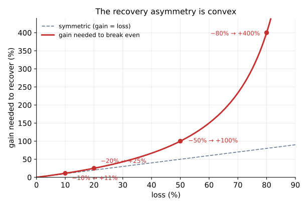
The gain needed to break even, plotted against the loss. If recovery were symmetric it would track the dashed line. Instead it curves away: a 10% loss needs 11%, a 50% loss needs 100%, an 80% loss needs 400%. The deeper the hole, the more disproportionate the climb out, which is the same concavity seen from the other side.
Apply this to log-wealth:
$$\mathbb{E}[\ln(1+R)] \leq \ln(1 + \mathbb{E}[R])$$
Here $R$ means the return in one period. If you gain 10%, then $R = 0.10$. If you lose 20%, then $R = -0.20$. The expression $1+R$ is your wealth factor, the number your money gets multiplied by over that period.
This expression only makes sense when $1+R > 0$. Returns below $-100%$ are outside the model because they correspond to ruin.
The left side is the average log-growth rate, which is what determines long-run compounding. The right side is the log of one plus the average return. The inequality is strict whenever returns vary. If returns were perfectly constant, the two sides would be the same. Variability is what creates the gap.
That distinction matters. The Jensen gap is the general geometric fact. Variance drag is the second-order approximation to that fact when returns are not too large.
To estimate the size of the gap, expand $\ln(1+R)$ in a Taylor series around the mean return $\mu$:
$$\ln(1+R) \approx \ln(1+\mu) + \frac{R-\mu}{1+\mu} - \frac{(R-\mu)^2}{2(1+\mu)^2} + …$$
Now take expectations term by term. Because $\mu = \mathbb{E}[R]$, we have $\mathbb{E}[R-\mu] = 0$, so the linear term vanishes. And because $\sigma^2 = \mathbb{E}[(R-\mu)^2]$, the quadratic term becomes the variance. That gives:
$$\mathbb{E}[\ln(1+R)] \approx \ln(1+\mu) - \frac{\sigma^2}{2(1+\mu)^2}$$
For small returns, and therefore for $|\mu| \ll 1$, we can use $\ln(1+\mu) \approx \mu$ and $(1+\mu)^2 \approx 1$. Then this simplifies to:
$$G \approx \mu - \frac{\sigma^2}{2}$$
Here $\mu$ is the arithmetic mean return, $\sigma^2$ is the variance of returns, and $G$ is the approximate geometric growth rate. So the geometric growth rate is approximately equal to the arithmetic mean $\mu$ minus half the variance. Variance drag is literally the second-order term in the Taylor expansion of a concave function.
This is Jensen’s inequality showing up in a form that is easy to compute. Because the logarithm is concave, variance lowers expected log-return. A portfolio with $\mu = 10%$ and $\sigma = 20%$ has geometric growth of approximately $8%$, which means a 2% annual drag from volatility alone.
In continuous-time finance, the same effect appears as the Itô correction term in geometric Brownian motion. That is why expected log-growth sits below arithmetic drift by roughly $\sigma^2/2$ there as well.
If you write wealth as
$$\frac{dW_t}{W_t} = \mu,dt + \sigma,dB_t$$
then Itô’s lemma gives
$$d\ln W_t = \left(\mu - \frac{\sigma^2}{2}\right)dt + \sigma,dB_t$$
The drift term for log-wealth is not $\mu$ but $\mu - \sigma^2/2$. In other words, the same “variance drag” that appeared above as a local Jensen effect shows up exactly in the canonical continuous-time model of finance.
If you want to see the difference numerically, a simple path simulation makes the gap visible:
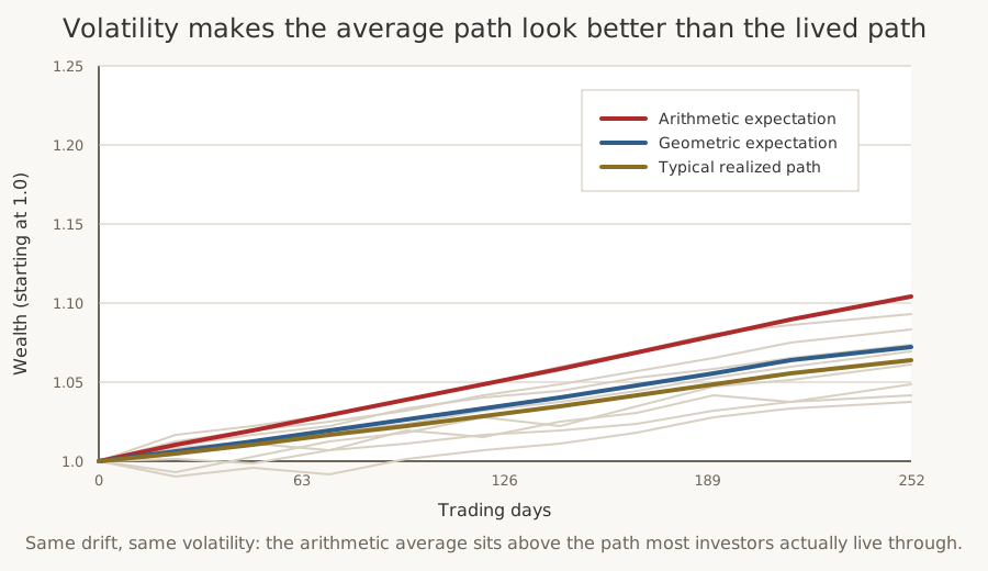
The red line is the arithmetic expectation. The blue line is the geometric expectation. The gold line tracks a more typical realized path. The faint gray lines are sample paths. They all start from the same wealth, but the arithmetic average drifts above the path most investors actually live through.
The exact numbers vary by run, but the pattern is stable: arithmetic averages look better than geometric ones, and median terminal wealth typically sits below the arithmetic mean because compounding punishes volatility path by path.
#V. Kelly’s Criterion: Optimization Under Concavity
Kelly’s criterion is the optimization consequence of the geometry just described. Jensen’s inequality says the concavity of the logarithm penalizes variance. Kelly asks: given that penalty, what exposure level maximizes expected log-growth? The answer puts variance directly in the denominator.
Long before Kelly, Daniel Bernoulli had already moved in the right direction. In 1738, in his analysis of the St. Petersburg paradox, he proposed logarithmic utility. He did not frame it in terms of time averages or ergodicity, but he correctly saw that the value of money is not linear and that multiplicative risk changes the problem.
Claude Shannon’s work is foundational here. In 1948, Shannon created information theory, a mathematical framework for reasoning about signal, noise, and transmission. The deep idea is that information can be measured, that uncertainty has structure, and that better information changes what an optimal repeated decision looks like. That is the intellectual foundation Kelly stands on.
In Shannon’s framework, information has operational value because it improves your ability to act under uncertainty. Kelly’s central insight was to take that logic and apply it to betting and capital allocation. If information improves the quality of your edge, then there is an optimal way to convert that edge into compounded wealth growth.
In 1956, John Larry Kelly Jr., a researcher at Bell Labs, derived the optimal betting strategy for a gambler with a private wire giving him noisy information about horse races. His derivation came directly from Shannon’s information theory, the mathematics of signal transmission through noisy channels.
Kelly maximized the expected logarithm of wealth because wealth compounds multiplicatively, and the logarithm converts this into additive growth rates that can be averaged over time.
The Kelly criterion maximizes:
$$G = \mathbb{E}[\ln(W_t/W_{t-1})]$$
Here $W_t$ means your wealth at time $t$. So $W_t/W_{t-1}$ is simply “how much your wealth changed this period,” and the logarithm turns that multiplicative change into something you can add across time.
For a simple bet with probability $p$ of winning, odds $b$, and probability $q=1-p$ of losing, the optimal fraction $f^*$ of wealth to bet is:
$$f^* = \frac{pb - q}{b} = \frac{p(b+1) - 1}{b}$$
For continuous returns, where $\mu$ is the expected return, $r$ is the risk-free rate, and $\sigma^2$ is the variance, the Kelly fraction becomes:
$$f^* = \frac{\mu - r}{\sigma^2}$$
Notice what appears in the denominator: variance. Kelly’s formula explicitly shows that optimal position size depends on the ratio of edge to variance. A strategy with twice the edge but twice the variance gets the same allocation as the original. Variance does more than measure “risk” here; it sets the size of the optimal position directly.
Under the usual favorable-bet assumptions, Kelly betting grows wealth faster than any other fixed-fraction strategy in the long run, dominating the alternatives with probability approaching 1 as time goes to infinity.
Edward O. Thorp was the person who carried this from theory into practice. He used Kelly-style reasoning first in blackjack and then in markets, showing that log-optimal sizing was a workable decision rule under uncertainty as well as an elegant theorem.
Leo Breiman gave the result one of its clearest mathematical statements. In 1961, he showed that the log-optimal strategy asymptotically dominates alternative strategies under broad conditions. Kelly gave the rule. Thorp made it operational. Breiman helped make the long-run claim precise.
Thomas Cover pushed the idea further. His work on universal portfolios showed that you can approach the long-run performance of the best constant-rebalanced portfolio in hindsight without knowing the true return distribution in advance. This extends the Kelly logic from “what is the optimal fraction if I know the edge?” to “how do I adapt toward log-optimal growth when the world is uncertain and my estimates are imperfect?” It is one of the cleanest bridges between growth optimality and learning.
Robert Fernholz extended the geometric view in a different direction through stochastic portfolio theory. His contribution was to show that relative portfolio performance can emerge from market structure itself, diversity, rebalancing, and the geometry of capital flows, not just from forecasting expected returns. It reinforces the same point: in a multiplicative world, portfolio results are shaped by pathwise structure and compounding mechanics, not only by static one-period expectations.
#Fractional Kelly
Practitioners rarely use full Kelly. The optimal fraction maximizes growth rate but produces extreme volatility, and drawdowns of 50% or more are common. Instead, they use half-Kelly or quarter-Kelly:
$$f_{half} = \frac{f^*}{2}$$
Under the standard local approximation around the Kelly optimum, this reduces growth rate by about 25% but cuts volatility in half. It also provides a safety margin against estimation error. If your estimate of $\mu$ or $\sigma$ is wrong, full Kelly can be catastrophic. Fractional Kelly is the recognition that maximizing geometric growth is the goal, but estimation uncertainty requires humility.
#VI. Ergodicity Economics: Time vs. Ensemble
In 2019, physicist Ole Peters published a paper in Nature Physics that should have forced a much sharper debate about the foundations of decision theory. Peters is one of the central modern figures in this article’s argument because he redefines the objective instead of adding another risk model. His broader research program, including earlier work with Alexander Adamou, showed that expected utility theory, the foundation of modern economics, rests on the implicit assumption of ergodicity.
To understand the force of that critique, it helps to name the benchmark. In 1944, John von Neumann and Oskar Morgenstern formalized expected utility theory in Theory of Games and Economic Behavior. Their framework asks which action maximizes average utility across possible states of the world. It became the dominant mathematical language of rational choice. The Peters critique is aimed at this formal benchmark, not at a vague intuition.
A process is ergodic if the time average equals the ensemble average. In ergodic systems, averaging across many parallel realizations gives the same long-run result as following one realization through time.
Wealth growth is not ergodic. Consider a gamble that multiplies your wealth by $1.5$ on heads and by $0.6$ on tails, each with probability one half. Averaged across many people betting in parallel, wealth grows: the ensemble average factor is $0.5 \times 1.5 + 0.5 \times 0.6 = 1.05$, a 5% gain per round. But a single person betting repeatedly almost surely goes broke, because the time-average growth factor is $\sqrt{1.5 \times 0.6} = \sqrt{0.9} \approx 0.95$, a loss of about 5% per round. The ensemble looks like a winning bet. The lived path is ruin.
This is where the distinction between ensemble optimality and pathwise optimality becomes decisive. A strategy can look optimal when you average across many parallel worlds, yet still be disastrous for one person living through one realized sequence of outcomes.
In the Peters-Adamou framing, standard expected-utility theory evaluates choices across possible states of the world, while individual investors experience one path through time. They cannot access parallel universes where they both survived and went bankrupt.
Adamou’s contribution matters here because the joint Peters-Adamou work did more than restate the ergodicity objection in the abstract: it used specific paradoxes, especially the St. Petersburg paradox, to show how changing the time resolution of the problem changes what counts as a rational decision. That made the time-average interpretation concrete rather than merely philosophical.
The correction is simple: maximize the time-average growth rate. This is exactly Kelly’s criterion. The logarithmic utility that Daniel Bernoulli invented to solve the St. Petersburg paradox in 1738 was correct, but economists forgot why: it emerges naturally from the non-ergodicity of multiplicative growth.
Jensen’s inequality is what makes the two averages different. Because the logarithm is concave, expected log-growth (the time average) is always less than the log of expected growth (the ensemble average). The gap between them is the Jensen gap from Section IV. Non-ergodicity is what turns that gap into a matter of survival rather than a technicality: you compound along one path, not across all possible paths.
This also clarifies the limit of mean-variance thinking. Markowitz’s framework is useful as a first approximation, but it treats risk as a tradeoff between average return and dispersion in a single period. It does not, by itself, encode the asymmetry of compounding through time or the special importance of ruin.
Paul Samuelson spent years arguing against overextending Kelly logic. His objections were not trivial; they forced the distinction between maximizing expected utility and maximizing long-run growth into the open. Even if one ultimately sides with Kelly and Peters for multiplicative wealth, Samuelson is part of the reason the debate became intellectually sharp.
#VII. Absorbing Barriers and the River
Taleb’s river analogy makes the mathematics visceral:
Never cross a river that is on average four feet deep.
If the river is eight feet deep in the middle and dry on the sides:
- Arithmetic mean: $(0 + 8)/2 = 4$ feet, which seems safe
- Actual constraint: if you are shorter than eight feet, the deep section still kills you
The river’s average depth is irrelevant. What matters is whether any point along the path is deep enough to kill you. The same logic applies to multiplicative wealth: a single ruinous outcome matters more than an average taken across hypothetical parallel paths.
Mathematically, zero is an absorbing barrier. If wealth hits zero, the process stops. You cannot recover. The arithmetic mean ignores this because it averages across paths where you survived and paths where you died. The geometric mean, via the logarithm, assigns infinite negative utility to zero: $\ln(0) = -\infty$.
This is why log-optimal sizing heavily penalizes strategies that expose you to ruin. The logarithm’s concavity makes ruin infinitely worse than any potential gain can compensate for, which is why practical Kelly sizing is always constrained by the possibility of catastrophic loss.
#VIII. Fat Tails and Higher Moments
The Taylor expansion of $\ln(1+R)$ does not assume normality; it is a local expansion that is useful when returns are small enough and the relevant moments exist. But financial returns live in Extremistan (Taleb’s term for domains governed by fat-tailed distributions), where extreme events are far more likely than the normal distribution predicts.
Mathematician Benoit Mandelbrot is the foundational figure here. Long before Taleb, Mandelbrot argued that speculative prices do not behave like neat Gaussian variables. They jump, cluster, and produce extreme moves far more often than classical models would suggest. Once that is true, the simple variance-based approximation is no longer enough. The tails start to dominate the economics.
Physicist Jean-Philippe Bouchaud pushed this critique further by arguing that the standard equilibrium picture of markets is too clean. His distinct contribution is to connect fat tails to market microstructure and crowd dynamics. Prices are shaped by crowding, feedback, market impact, and institutional structure, as well as by distributions around a stable mean. Tail risk is built into how markets actually work, not merely a statistical annoyance.
Physicist Didier Sornette adds another layer. He models bubbles and crashes as endogenous critical phenomena generated by positive feedback, imitation, and unstable market structure. In his framework, some of the biggest crashes are the natural end point of a system that has become reflexive and fragile, not random bolts from the blue.
When returns are fat-tailed, higher moments matter. The cleanest way to see that is to expand the logarithm directly around $R=0$. For $|R|<1$,
$$\ln(1+R) = R - \frac{R^2}{2} + \frac{R^3}{3} - \frac{R^4}{4} + …$$
Taking expectations gives
$$\mathbb{E}[\ln(1+R)] = \mathbb{E}[R] - \frac{1}{2}\mathbb{E}[R^2] + \frac{1}{3}\mathbb{E}[R^3] - \frac{1}{4}\mathbb{E}[R^4] + …$$
This version is more explicit than the shorthand mean-variance formula. The second moment enters with a negative sign, so dispersion hurts growth. The third raw moment enters with a positive sign, which is why positive skew tends to help and negative skew tends to hurt. The fourth raw moment also enters with a negative sign, which means that large extreme moves, whether positive or negative, reduce expected log-growth unless they are offset elsewhere in the distribution. In practice, that means the simple mean-and-variance picture stops being enough once extreme moves become common.
Strictly speaking, these are raw moments, not skewness and kurtosis themselves. But the intuition lines up with the standardized versions: asymmetry matters, and tail thickness matters. If you wanted to write the same logic more cleanly, cumulants would often be the better language. The point is the same either way: once higher moments become large, the mean-variance shorthand loses explanatory power.
Standard option pricing models (Black-Scholes) assume log-normal returns with thin tails. In practice, traders partially correct for this with volatility smiles and skews, but any framework that stays too close to a thin-tailed world will still understate the probability of extreme moves. The exact crash frequency matters less than the broader implication: left-tail events occur materially more often than a naive Gaussian calibration suggests.
Taleb’s barbell strategy is the practical philosophical response to this entire section. His central point goes past the claim that tails are fatter than standard models admit: the right response to a fat-tailed world is to organize a portfolio so that ordinary outcomes are survivable and extraordinary dislocations become opportunities rather than existential threats. A barbell does exactly that: most of the capital sits in positions that are robust to ordinary noise, while a small allocation buys extreme convexity.
That structure matters because it changes the shape of the return distribution itself. The puts have bounded downside (premium paid) and very large upside in crashes. That creates positive skewness, limits exposure to ruinous left-tail states, and preserves the possibility of large gains when the system breaks. In Jensen-Kelly terms, Taleb’s contribution is to insist that the objective is to survive and compound in a discontinuous world, not to maximize a smooth average in a well-behaved one.
Economist Hyman Minsky belongs in this picture too. His core idea was that stability breeds fragility. Long calm periods encourage leverage, maturity mismatch, and crowded positioning, which makes the eventual break far more violent. That is exactly the kind of environment where average outcomes look benign right up until the left tail arrives. Mandelbrot, Bouchaud, Sornette, and Minsky all push in the same direction: the left tail is part of the structure of the world itself, not a small correction to a calm baseline.
It is worth being precise about what is doing the work here, because two facts are at play, not one. Concavity, the Jensen effect, says variability is costly. Fat tails say the variability is larger and more one-sided than a Gaussian world assumes. The first is geometry; the second is a fact about the distribution that geometry acts on. Tail hedging matters because both are true at once: the penalty for dispersion is real, and the dispersion is bigger than the textbook admits.
#IX. The Put Strategy as Jensen-Optimal
Spitznagel’s tail hedge, 100% SPY plus deep OTM puts, is where the abstract logic becomes a concrete portfolio. It is best understood as two legs that do different jobs.
The growth engine. The first leg is full exposure to the market: 100% SPY. This is the part that compounds. Left alone it also carries the full left tail, and as the previous sections showed, the left tail is what does disproportionate damage to long-run growth. The growth engine supplies market exposure and most of the arithmetic return; by itself it does nothing about the variance drag and ruin risk that concavity imposes.
The convex overlay. The second leg is a small allocation to deep out-of-the-money puts. Most of the time they expire worthless. In a crash they pay many multiples of premium. Their job is to truncate the left tail, removing the states that compounding punishes most; adding return on average is not the point. This is the leg that addresses the geometry the rest of the article is about.
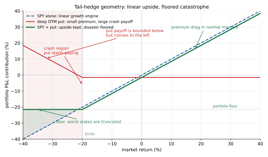
The two legs and their sum. SPY alone (blue) is pure linear exposure: it carries the full left tail. The deep OTM put (red) costs a small premium most of the time and pays off only in a crash. Add them and you get the overlay (green): it keeps the upside, minus the premium, but its left tail is floored. The growth engine compounds; the convex overlay removes the states that do the most damage to that compounding.
Rather than simply buying disaster insurance in the conventional sense, Spitznagel takes the full chain, compounding, concavity, variance drag, fat tails, and non-ergodicity, and turns it into a specific capital-allocation rule. That is why he is central to this argument rather than an optional practitioner example. Many investors understand the words “fat tails” and still build portfolios as though crashes are just unpleasant drawdowns around a stable mean. Spitznagel’s contribution is to force the implication all the way through: if the left tail dominates long-run outcomes, then convexity belongs inside the core architecture of the portfolio rather than bolted on as a cosmetic add-on.
Even in the simplest second-order approximation, the mechanism is clear. Recall the approximate growth formula:
$$G \approx \mu - \frac{\sigma^2}{2}$$
The two legs map onto the two terms. The growth engine supplies $\mu$. The overlay works on the second term:
- The cost: Puts have negative expected return, since they usually expire worthless. This reduces $\mu$ by the premium paid, say 0.5% annually.
- The benefit: In a crash, puts can pay off many multiples of premium, truncating the left tail. In a local approximation, that reduces the effective variance term. More importantly, it removes the states that are most destructive to future compounding.
Because the variance drag is quadratic in the local approximation, a modest reduction in tail risk can outweigh a linear premium cost. But that is the conditional part of the claim, and it is worth stating plainly. Jensen and Kelly explain why reducing left-tail damage can be worth paying for. They do not guarantee that any particular put is worth its price. The trade works only if convexity is cheap enough relative to the protection it buys, and only if it is implemented with discipline: strike selection, roll mechanics, sizing, and a read on how persistently the market underprices left-tail risk. The mathematics tells you what to look for. It does not promise that the market is currently offering it.
This is also where Taleb and Spitznagel meet. Taleb supplies the philosophical and statistical doctrine: avoid ruin, respect discontinuities, seek convexity. Spitznagel supplies the portfolio expression of that doctrine: keep the growth engine, then add a small convex structure that changes what happens in the worst states. The combination is what makes tail hedging more than a fear trade. It becomes a compounding strategy.
#X. Beyond Equities: Where Convexity Is Cheaper
The SPY put strategy works, but it may not be optimal. The same Jensen-Kelly logic applies wherever there is reliable asymmetry between calm and crisis:
- Rates: Central banks cut aggressively in crises (roughly 500bps over 2007–08, 150bps in two weeks during COVID). OTM calls on SOFR futures can capture these panic cuts at low carry cost, though stagflation breaks the thesis.
- FX carry: Currencies like AUD/JPY offer 3-5% annual carry that unwinds violently in risk-off events (AUD/JPY fell from above 104 in July 2008 to near 55 in October). The carry itself can fund OTM puts on the high-yielder.
- Credit: IG bonds earn spread, but credit events cluster. CDS protection is convex: IG CDX spreads moved from roughly 50bps to the mid-200s in 2008, while HY CDX moved from the low hundreds toward the 1,500–1,600bps region. The barbell is earn IG spread, buy HY CDS protection.
- Commodities: Oil grinds in a narrow range, then spikes above $140 or crashes into the $30s. Deep OTM strangles capture both tails, though supply shocks make crude a noisier hedge than the others.
The Universa insight is to scan across these markets for wherever tail convexity is cheapest right now. Sometimes that is equity vol, sometimes credit, sometimes rates. The previous article develops each market in more detail, with specific trade structures, counterexamples, and implementation notes.
#XI. How This Fits the Series
The previous three pieces in the Leptokurtic series looked separate, but they are all instances of the same structure. Twenty Centuries of Financial Data established the empirical backdrop: fat tails, devaluations, and regime shifts are the historical baseline, not modern anomalies. Detecting Crashes with Fat-Tail Statistics moved to live diagnostics, showing that crashes have detectable precursors and tail behavior that standard tools miss. The Tail Hedge Debate tested the put overlay on real SPY options data and found that deep out-of-the-money convexity can improve a portfolio’s realized path when funded and sized the way Spitznagel describes. Those three supplied the data, the diagnostics, and the implementation; this one supplies the mathematics that connects them.
It is worth being explicit about the division of labor. Jensen’s inequality is the geometric core, but it is not the whole story by itself. Jensen explains why concavity penalizes variability. Kelly turns that into a sizing rule. Non-ergodicity explains why the relevant objective is the time path rather than the ensemble average. Fat-tail theory explains why variance alone is often not enough because extreme states dominate the economics. The full argument works because these pieces fit together, not because one theorem replaces all the others.
#XII. The Full Intellectual Lineage
What looks like a single modern investing idea is actually a chain in which each figure adds one missing piece, or corrects one mistake, left by the previous framework. It runs in two strands, each roughly chronological on its own: first the classical construction of growth-optimal investing, then the modern reckoning with fat tails, fragility, and time.
#The construction: logarithms, growth, and optimal sizing
-
Napier (1614): Napier gives the first indispensable tool. Logarithms linearize multiplicative processes, so $\log(ab) = \log(a) + \log(b)$. Without that move, there is no clean way to turn compounding into something that can be analyzed additively.
-
Jacob Bernoulli (1680s): Bernoulli studies the limit later denoted by $e$. That connects Napier’s logarithmic tool to continuous compounding. Napier gives the language. Bernoulli identifies the natural constant that belongs to that language.
-
Daniel Bernoulli (1738): Daniel Bernoulli is the first major bridge from pure mathematics to decision theory. He takes the logarithm and applies it to risky choice, arguing that multiplicative risk changes rational behavior. He does not yet have Kelly or ergodicity, but he points in their direction.
-
Jensen (1906): Jensen supplies the missing geometric theorem. If the relevant function is concave, variability is penalized. That turns Daniel Bernoulli’s logarithmic intuition into a general structural fact: once wealth is evaluated through a concave function, randomness has a systematic cost.
-
von Neumann and Morgenstern (1944): They formalize expected utility as the dominant benchmark for rational choice. This is the framework that later thinkers will refine, challenge, or partially reject. Their role is not to solve the compounding problem. Their role is to define the benchmark that Peters will later criticize.
-
Shannon (1948): Shannon makes uncertainty operational. Information is measurable, noise has structure, and better signals change what an optimal repeated decision looks like. This is the mathematical foundation that Kelly later turns into a capital-allocation rule.
-
Markowitz (1952): Markowitz gives finance a tractable one-period approximation through mean-variance analysis. That is a real advance, but it is also a simplification. He makes portfolio choice practical, while leaving compounding, path dependence, and ruin underemphasized.
-
Kelly (1956): Kelly takes Shannon’s information-theoretic framework and translates it into repeated betting and investment. He shows how an edge should be converted into position size when the objective is long-run compound growth. This is where logarithms, information, and compounding become one explicit rule.
-
Thorp and Breiman (1961 onward): Thorp shows Kelly can be used in practice, and Breiman gives the long-run dominance result mathematical force.
-
Cover (1991): Cover extends the growth-optimal tradition into learning. Universal portfolios show that even without a fully known model, it is possible to asymptotically approach the performance of the best rebalanced portfolio in hindsight. This makes the Kelly logic more robust under model uncertainty.
-
Fernholz (2002): Fernholz extends the geometric tradition into portfolio construction itself. Stochastic portfolio theory shows that diversity, rebalancing, and market structure can generate relative returns even without heroic forecasting. That broadens the argument from optimal sizing to the geometry of portfolio design.
#The reckoning: fat tails, fragility, ergodicity, and practice
-
Mandelbrot (1963): Mandelbrot challenges the statistical comfort behind standard finance. Returns are not well described by thin-tailed Gaussian assumptions. Once that is true, simple mean-variance reasoning becomes less reliable, and the left tail matters much more.
-
Samuelson (1969): Samuelson is the critic who forces the distinction between expected utility and long-run growth to be stated clearly.
-
Minsky (1986): Minsky adds the macro-financial mechanism: stability breeds fragility, so left-tail risk is generated by the system itself.
-
Bouchaud (2003 to 2008): Bouchaud links fat tails to market microstructure, feedback, and crowd behavior.
-
Sornette (2003): Sornette models bubbles and crashes as endogenous critical phenomena rather than exogenous shocks.
-
Taleb (2007 to 2012): Taleb is where the statistical critique of fat tails becomes a doctrine of survival. Ruin, fragility, convexity, and asymmetry stop being technical side notes and become the core portfolio problem. Mandelbrot tells you the tails are fatter than you think. Taleb tells you that once you accept that fact, the whole logic of risk-taking has to change.
-
Peters and Adamou (2011 to 2019): Peters and Adamou reopen the foundations of decision theory by showing that non-ergodic multiplicative processes must be evaluated along time paths, not across hypothetical ensembles. This reconnects Kelly to a deeper justification: more than a clever betting rule, it is the correct objective for a non-ergodic compounding process.
-
Spitznagel (2021): Spitznagel is the implementation layer. He takes the whole chain, logarithms, concavity, Kelly sizing, fat tails, fragility, and non-ergodicity, and turns it into a practical portfolio architecture built around convex protection and survival through crashes. He is the point where the mathematics ceases to be interpretation and becomes an actual portfolio design.
#Conclusion: The Geometry of Survival
Jensen’s inequality is the geometry of survival in a multiplicative world, not a mathematical curiosity. Wealth is organized by ratios, not differences, and the logarithm is the coordinate system that makes that structure visible. Because that coordinate change is concave, volatility is geometrically destructive: a quadratic drag on compound growth.
The long confusion in economics was treating the ensemble average as if it were the investor’s lived path. The arithmetic mean looks at what happens across a population of investors in parallel. The geometric mean looks at what happens to you through time. For a single investor compounding over decades, only the time average matters.
Tail hedging works because it respects this geometry. It accepts a small, certain reduction in arithmetic return (the put premium) in exchange for protection against the states that do the most damage to compound growth. In a local approximation, that looks like paying to reduce a quadratic variance penalty. In the fuller fat-tailed picture, it is better understood as paying to reduce exposure to ruinous left-tail paths.
The logarithm was invented to help astronomers multiply. Four hundred years later, it reveals why crash insurance can be worth paying for, and why, when returns compound, survival comes before growth.
#References
- Bernoulli, D. (1738). “Specimen Theoriae Novae de Mensura Sortis.”
- Bernoulli, J. (1685). Ars Conjectandi (posthumous, 1713)
- Bouchaud, J. P. & Potters, M. (2003). Theory of Financial Risk and Derivative Pricing. Cambridge University Press.
- Bouchaud, J. P. (2008). “Economics Needs a Scientific Revolution.” Nature, 455.
- Breiman, L. (1961). “Optimal Gambling Systems for Favorable Games.”
- Cover, T. M. (1991). “Universal Portfolios.” Mathematical Finance, 1(1).
- Fernholz, R. (2002). Stochastic Portfolio Theory. Springer.
- Jensen, J. L. W. V. (1906). “Sur les fonctions convexes et les inégalités entre les valeurs moyennes.” Acta Mathematica, 30.
- Kelly, J. L. (1956). “A New Interpretation of Information Rate.” Bell System Technical Journal, 35(4).
- Mandelbrot, B. (1963). “The Variation of Certain Speculative Prices.” The Journal of Business, 36(4).
- Mandelbrot, B. & Hudson, R. L. (2004). The (Mis)Behavior of Markets. Basic Books.
- Markowitz, H. (1952). “Portfolio Selection.” The Journal of Finance, 7(1).
- Minsky, H. P. (1986). Stabilizing an Unstable Economy. Yale University Press.
- Napier, J. (1614). Mirifici Logarithmorum Canonis Descriptio
- Peters, O. & Adamou, A. (2011). “The Time Resolution of the St Petersburg Paradox.” Philosophical Transactions of the Royal Society A, 369(1956).
- Peters, O. & Gell-Mann, M. (2016). “Evaluating Gambles Using Dynamics.” Chaos, 26(2).
- Peters, O. (2019). “The Ergodicity Problem in Economics.” Nature Physics, 15.
- Samuelson, P. A. (1969). “Lifetime Portfolio Selection by Dynamic Stochastic Programming.”
- Shannon, C. E. (1948). “A Mathematical Theory of Communication.” Bell System Technical Journal, 27.
- Sornette, D. (2003). Why Stock Markets Crash. Princeton University Press.
- Sornette, D. (2017). Why Stock Markets Crash: Critical Events in Complex Financial Systems (updated edition). Princeton University Press.
- Spitznagel, M. (2021). Safe Haven: Investing for Financial Storms. Wiley.
- Taleb, N. N. (2007). The Black Swan: The Impact of the Highly Improbable. Random House.
- Taleb, N. N. (2012). Antifragile: Things That Gain from Disorder. Random House.
- Thorp, E. O. (1997). “The Kelly Criterion in Blackjack, Sports Betting, and the Stock Market.”
- von Neumann, J. & Morgenstern, O. (1944). Theory of Games and Economic Behavior. Princeton University Press.
From the series Leptokurtic.
Written with an LLM in the loop, like everything here. The ideas and the mistakes are mine. More on how I write.