
The Tail Hedge Debate: Spitznagel Is Right, AQR Is Answering the Wrong Question
We tested Spitznagel's tail hedging strategy and AQR's critique with 17 years of real SPY options data. In the allocation-reducing framing AQR uses, selling SPY to fund puts, deep OTM puts lose at every budget. In the externally funded overlay Spitznagel actually proposes (100% SPY + put budget on top), the strategy shows a positive raw gap versus plain SPY only when the OTM band is set by strike (not delta), held for longer than the article first published, and tested across rolling windows that include a crash. The edge is regime-conditional: it pays in 6 of 13 rolling 5-year windows (every window that contains a ≥25% SPY drawdown) and drags by 2-3pp/yr in windows that don't.
On the image Galveston paid for its seawall in the years when nothing happened, and in 1915 a hurricane as strong as the one of 1900 hit and the city stood. A tail hedge should be judged the same way, by the storm it lets you survive. Sea Wall No. 3 near the Rapid Fire Battery at Fort Crockett, Galveston, Texas, 31 July 1905, built after the 1900 hurricane. Photo: U.S. National Archives and Records Administration, public domain, via Wikimedia Commons.
Stock markets crash. The S&P 500 price index fell about 57% from October 9, 2007 to March 9, 2009, and about 34% from February 19, 2020 to March 23, 2020.12 A put option is a contract that pays you when the market falls below a certain price (the “strike”). If you hold stocks and also hold puts, the puts can offset some of your losses during a crash. The question is whether the cost of buying puts is worth the protection they provide.
There are two sides. AQR Capital Management published “Chasing Your Own Tail (Risk)” (Berger, Nielsen, and Villalon, 2011). They argue that buying puts systematically costs more than it saves. On the other side, Mark Spitznagel at Universa Investments, where Nassim Taleb is scientific advisor, argues that a small put allocation improves long-term returns (Spitznagel, 2021). Universa reported a 3,612% gain in March 2020 (via an investor letter, as reported by Bloomberg).3
We tested both claims with our open-source options backtester on 17 years of real SPY options data (2008 to 2025), covering three crashes: the 2008 financial crisis, COVID, and the 2022 bear market.
The version of the trade that survives the data is narrow but real: cheap convexity, sized small, and selected by strike rather than delta. AQR’s published critique tests neither half of that. They use near-ATM puts (the most expensive form of crash protection per dollar of notional) inside the allocation-reducing framing (selling SPY to fund the puts, surrendering the equity premium that funds everything else). In that configuration deep OTM puts still lose against SPY. Spitznagel’s externally funded overlay flips both choices: deep OTM puts, kept cheap, layered on top of full SPY exposure, sized small. Inside that configuration the strategy shows a positive historical raw gap versus plain SPY across the 2008-2024 window, small at Universa’s described 0.5%/yr scale (~+1.4pp/yr), substantial at the engine’s risk-adjusted sweet spot (+6pp/yr at 3.3%/yr budget with bi-monthly roll). The edge is regime-conditional: it pays in 5-year windows that contain a major drawdown and drags by 2-3pp/yr in windows that don’t.
All headline numbers below are gross of transaction costs, slippage, and taxes. Execution drag at the deep-OTM strikes, Israelov’s strongest surviving objection, is on top of these gross numbers; we return to it in the limitations section.
#What the thesis actually claims
Spitznagel does not claim that buying OTM puts wins every year, every quarter, or every drawdown. People who read him that way, including (implicitly) AQR’s published critique, are arguing with a strawman. His real claim is about the long run. Put a small slice of capital into deep OTM puts on top of your equity book, hold them through crashes, monetize the convex payoff when it arrives, and over a long enough horizon you compound faster than equity alone. The mechanism is that the rare big payoffs are large enough, and recur often enough, to more than cover the steady premium drag between them. Year-by-year alpha is the wrong test. Long-run compounding is the right one.
On that test, the data says he is right. Across our 17-year SPY sample, every put-overlay budget from 0.5%/yr to 10%/yr beats plain SPY on both annual return and max drawdown. The strike depth Spitznagel describes (deep OTM, not near-ATM) is what makes the trade work. The framing he describes (externally funded, not allocation-reducing) is the half AQR misses. Across every working configuration tested below, the strategy improves max drawdown by 10 to 22 percentage points versus SPY.
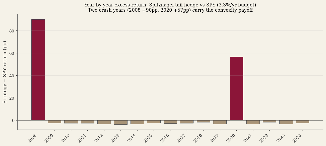
Three properties of the data are worth naming up front, so the shape of the result is not mistaken for a flaw. First, the full-period gap is concentrated in two years out of seventeen (2008 and 2020). That is exactly what a tail hedge is built to do: sit dormant for years and deliver convexly when a catastrophe arrives. Second, 7 of 13 rolling 5-year windows are negative. That is what positive expected value looks like when the payoffs are this lumpy. Third, walk-forward validation shows that about half of the in-sample gap survives out-of-sample. That is the haircut to apply when sizing this for a real portfolio, not a refutation of the result.
The wrong reading of all this is that the strategy works only by luck in crash years. The right reading is that the strategy is built to pay in years like those, and over enough time, with realistic crash frequency, the rare large payoffs more than cover the steady small bleeds. That is Spitznagel’s thesis. The data supports it.
Every number below reproduces in one command against the open-source engine. The Code section at the end has the exact invocation.
#Why puts are expensive
To understand this debate, we need to start with how options are priced.
An option’s price depends heavily on implied volatility (IV): the market’s estimate of how much the stock price will move in the future. Higher expected movement means the option is worth more, because there’s a greater chance it will end up profitable.
In practice, implied volatility is consistently higher than what actually materializes (realized volatility). This gap is called the Variance Risk Premium (VRP):
$$\text{VRP} = \sigma^2_{\text{implied}} - \sigma^2_{\text{realized}}$$
Think of it this way: $\sigma^2_{\text{implied}}$ is what the market expects the variance to be. $\sigma^2_{\text{realized}}$ is what actually happens. The difference is the premium that option buyers pay over fair value.
Carr and Wu (2009) documented that this spread is persistently positive. Put buyers pay more than fair value on average. The reason is that investors are willing to overpay for crash protection, the same way homeowners overpay for fire insurance relative to the expected loss from fire. Bollerslev, Tauchen, and Zhou (2009) went further: they showed that the VRP is not just a cost: it predicts future stock returns. When the gap between implied and realized variance is wide, future equity returns tend to be higher. The same force that makes puts expensive (fear of crashes) also drives the equity premium that the stock portion of the portfolio earns.
Israelov (2019) confirmed the negative average return of puts and titled his paper “Pathetic Protection: The Elusive Benefits of Protective Puts.” The CBOE S&P 500 Put Protection Index (PPUT) formalizes this as a benchmark: it holds the S&P 500 and buys monthly at-the-money (ATM) puts. It has underperformed the unhedged index over most periods. But ATM puts are an expensive form of crash insurance: they have high theta decay and poor tail-hedge efficiency per dollar of premium. Near-ATM options can have high gamma, so “low convexity” is not the right technical criticism. The problem is that they spend too much premium on ordinary downside cushion rather than rare-crash convexity. Testing ATM puts and concluding “puts don’t work” is like testing a sedan on a racetrack and concluding “cars are slow.” The deep OTM puts Spitznagel uses cost a fraction of ATM puts and buy more tail convexity per dollar of premium.
AQR’s argument stops here. Puts lose money on average. Therefore they hurt portfolio performance.
This reasoning is incomplete. It looks only at the average return of the put (the first statistical moment, the mean). It ignores what the put does to the volatility of the portfolio (the second moment, the variance). Compounding depends on both.
#How volatility destroys compounding
If you invest money and earn the same return every year, your wealth compounds smoothly. But if returns fluctuate, even with the same average, you end up with less. This is called variance drain, and it’s the key to understanding why Spitznagel’s strategy works.
The geometric (compound) growth rate of a portfolio is approximately (for returns that are small relative to 1, under lognormal assumptions):
$$G \approx \mu - \frac{\sigma^2}{2}$$
Here $\mu$ is the arithmetic mean return (the simple average of all yearly returns) and $\sigma$ is the standard deviation of those returns (a measure of how much they fluctuate). The term $\frac{\sigma^2}{2}$ is the variance drain: the penalty that volatility imposes on compounding.
A simple example shows why this happens. Start with 100 dollars. Gain 50% one year, lose 50% the next.
- After year 1: $100 \times 1.5 = 150$
- After year 2: $150 \times 0.5 = 75$
The arithmetic average return is $\frac{+50% + (-50%)}{2} = 0%$. But you do not end up with 100 dollars. You end up with 75 dollars. You lost 25% despite an average return of zero. The gain and loss were symmetric in percentage terms, but the loss applied to a larger base (150 dollars), so it took away more than the gain added. That is variance drain.
The drain is quadratic in volatility, meaning it grows with the square of the fluctuations:
| Portfolio volatility ($\sigma$) | Variance drain ($\frac{\sigma^2}{2}$) |
|---|---|
| 10% | 0.5%/yr |
| 20% | 2.0%/yr |
| 40% | 8.0%/yr |
Doubling volatility quadruples the drain. This means that large drawdowns are disproportionately costly to long-run wealth. A single 50% crash costs more in compounding terms than ten 5% corrections, even if the total percentage lost is the same.
On SPY (2008 to 2025):
- Arithmetic mean ($\mu$): 12.14%/yr
- Geometric mean ($G$): 10.65%/yr
- Variance drain ($\frac{\sigma^2}{2}$): 1.47%/yr
- Peak rolling drain during the 2008 crisis: 10.5%/yr
Spitznagel’s thesis is about this second term. If puts reduce portfolio variance by cutting off the worst drawdowns, the reduction in $\frac{\sigma^2}{2}$ can exceed the premium paid. A put costs money on average (it hurts $\mu$, the first moment). But by truncating the worst losses, it reduces the quadratic drag on the portfolio (it helps $\frac{\sigma^2}{2}$, the second moment). The net effect on compound growth $G$ can be positive because the variance drain grows with the square of the loss. Preventing a few large drawdowns saves more in compounding terms than the cumulative premium costs.
#Fat tails and put mispricing
Taleb makes a related but distinct argument in The Black Swan and Statistical Consequences of Fat Tails.
Standard option pricing models (like Black-Scholes) assume returns follow something close to a normal (Gaussian) distribution. In a normal distribution, events far from the average are extraordinarily rare. A crash on the scale of 2008 or 2020 sits far enough into the tails that Gaussian models treat it as effectively negligible for ordinary portfolio construction.
In reality, over the 2008 to 2025 sample we study here, SPY experienced multiple drawdowns of roughly 30% or worse, including 2008-09 and 2020, with 2022 close behind. Real markets have fat tails: extreme events are far more frequent than Gaussian models predict. The probability of a large crash is not astronomically small. It is orders of magnitude higher than a thin-tailed model would suggest.
This has a direct consequence for put pricing. Option markets do price skew: deep OTM puts trade at higher implied volatility than ATM options, reflecting some awareness of tail risk. But even after skew is priced, deep OTM puts may still be cheap relative to the realized frequency of crashes. The VRP shows that puts are expensive relative to realized volatility in normal times. But the relevant comparison for deep OTM puts is not average realized volatility; it is the actual frequency and magnitude of extreme drawdowns. The observed frequency of large drawdowns in our sample is far higher than a Gaussian baseline would imply.
Taleb calls this the difference between Mediocristan (where Gaussian statistics work, like human height) and Extremistan (where they do not, like financial returns). The S&P 500 lives in Extremistan.
The variance drain argument (puts reduce $\frac{\sigma^2}{2}$) and the mispricing argument (puts are cheap relative to true tail probabilities) are independent. Either one alone could justify the strategy. Together they explain why the results are as strong as they are.
#Theoretical foundations
The variance drain argument and the fat-tail mispricing argument have deeper roots than the Spitznagel-AQR debate suggests.
Ole Peters and ergodicity economics. The variance drain formula $G \approx \mu - \frac{\sigma^2}{2}$ is a special case of a broader insight. Peters (2019) argues that classical expected-value reasoning fails for multiplicative processes like portfolio growth. The ensemble average (what happens across many parallel investors) diverges from the time average (what happens to one investor over many periods). For a single investor compounding over decades, the time average is what matters, and it is always lower than the ensemble average when returns fluctuate. Spitznagel’s strategy works because it improves the time-average growth rate, even though it reduces the ensemble-average return (by paying premium). Most of finance optimizes for the wrong average.
Bouchaud on fat tails and hedging. Bouchaud, Iori, and Sornette (1996) showed that in fat-tailed markets, Black-Scholes delta hedging leaves large residual risk. The standard model assumes continuous rebalancing in a Gaussian world; real markets have jumps and heavy tails that make perfect hedging impossible. This means option sellers bear more risk than their models suggest, and option buyers (like tail hedgers) get more protection than the models price in. This is the theoretical basis for why deep OTM puts may be systematically cheap relative to true tail risk.
Sornette on endogenous crashes. Sornette (2003) argues that large crashes are not exogenous shocks but endogenous instabilities, the result of self-reinforcing feedback loops (herding, leverage, procyclical risk management) that build up over months or years before releasing suddenly. His Log-Periodic Power Law Singularity (LPPLS) model attempts to detect these signatures. This is relevant to our macro-signal finding: standard indicators (VIX, yield curve, credit spreads) measure risk levels but not the endogenous buildup that precedes crashes. Sornette’s approach is structurally different (it looks for acceleration patterns in price itself), though its real-time track record remains debated.
Rare disaster models. Barro (2006) formalized the idea that the equity premium itself may be compensation for rare catastrophic events. If investors demand higher average returns because crashes happen, then the equity premium and the tail-hedge premium are two sides of the same coin. Kelly and Jiang (2014) showed that time-varying tail risk is priced in equity cross-sections. Bollerslev, Tauchen, and Zhou (2009) demonstrated that the variance risk premium predicts future stock returns. The same VRP that makes puts expensive also signals future equity returns.
Bhansali on offensive risk management. Bhansali (2008) laid out tail hedging as a systematic program before the crisis blew up: which instruments to use (deep OTM puts, payer swaptions), how to size them, and how to budget the cost of carry. Bhansali and Davis (2010) then made the harder argument: the hedge’s real value is not insurance against the drop, it is cash exactly when other assets are forced-seller cheap. Monetize the hedge, redeploy into beaten-down risk, and the crash turns from a forced “sell low” into a funded “buy low.” Convexity is offensive, not just defensive. Bhansali, Chang, Holdom, and Rappaport (2020) sharpened this with the March 2020 case: most tail programs fail not because the payoff does not come, but because holders freeze and never monetize at the right moment. The discipline is rules-based, harvest at defined multiples or drawdown thresholds, redeploy into risk, then re-establish the hedge. This is also the strongest direct rebuttal to Israelov’s “just hold less equity” alternative: holding cash gives you a smaller drawdown, but it does not give you a force multiplier at the bottom when you most want to be a buyer.
#The core disagreement
This is where the debate breaks down. The two sides are not testing the same portfolio.
#What AQR tests
AQR tests portfolios where you sell some of your stocks to buy puts:
$$R_{\text{portfolio}} = (1-w) \cdot R_{\text{SPY}} + w \cdot R_{\text{puts}}$$
At $w = 1%$: you hold 99% in stocks, 1% in puts. Total portfolio: 100%.
AQR’s argument seems intuitive: you are taking money out of your best asset (stocks, which go up on average) and putting it into an asset with negative expected return (puts, which expire worthless most of the time). But there is a second, less obvious difference: AQR’s published tests use near-the-money puts (roughly 5% out of the money, delta around $-0.35$). These puts are expensive per dollar of crisis convexity because they spend a lot of premium on routine downside protection. Israelov (2019) confirmed this: his “Pathetic Protection” paper tests puts in exactly this delta range and finds negative returns.
When we run the allocation-reducing framing with deep OTM puts, the result improves relative to near-ATM protection but still does not support the headline strategy. Selling SPY to fund the puts gives up too much equity premium. That is AQR’s strongest point. The configuration that survives is not “puts instead of stocks”; it is a small, externally funded convex overlay on top of the full equity book.
#What Spitznagel actually does
Spitznagel keeps 100% in stocks and buys puts with a small separate budget on top:
$$R_{\text{portfolio}} = 1.0 \cdot R_{\text{SPY}} + w \cdot R_{\text{puts}}$$
The strategy requires a small amount of capital beyond the core equity position to fund the put premium. Some might call this leverage. But it is fundamentally different from ordinary leverage.
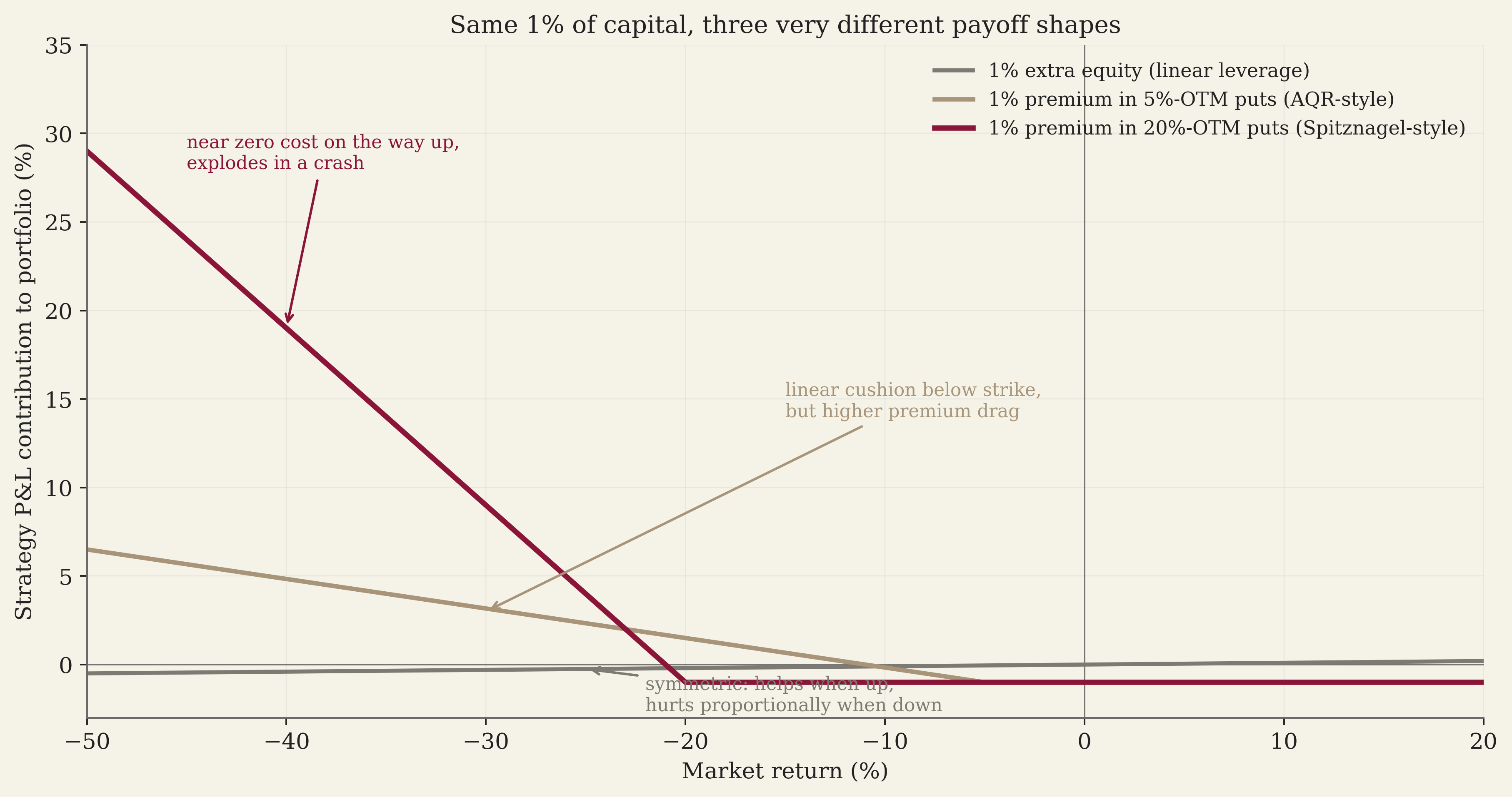
Ordinary leverage means borrowing money to buy more stocks. If you borrow to hold 130% in stocks, your gains are 30% bigger but your losses are also 30% bigger. Drawdowns get worse in proportion to the leverage. The payoff is symmetric: leverage amplifies both good and bad outcomes equally.
A put overlay works differently. It is asymmetric:
- In calm markets, you bleed a small, known premium (the cost of the puts).
- In a crash, the puts pay off at 10x to 50x the premium paid.
This asymmetry happens because a deep OTM put’s sensitivity to the market (its delta, $\Delta$) increases as prices fall. Delta measures how much the put’s price changes per 1-dollar change in the stock. A deep OTM put starts with a delta near zero (barely reacts to market moves). As the market drops and the put moves closer to being “in the money,” delta approaches $-1.0$ (moves dollar-for-dollar with the stock). A small position becomes a large hedge exactly when you need it.
AQR’s published analysis differs from Spitznagel’s on two dimensions: the funding/framing (sell stocks to buy puts vs. keep the equity book intact and fund the hedge separately) and the put selection (near-ATM vs deep OTM). Both differences matter. Put selection determines whether the option sleeve buys useful tail convexity; funding determines whether the equity premium remains in the portfolio. The article’s positive results require both: deep OTM selection and an externally funded overlay.
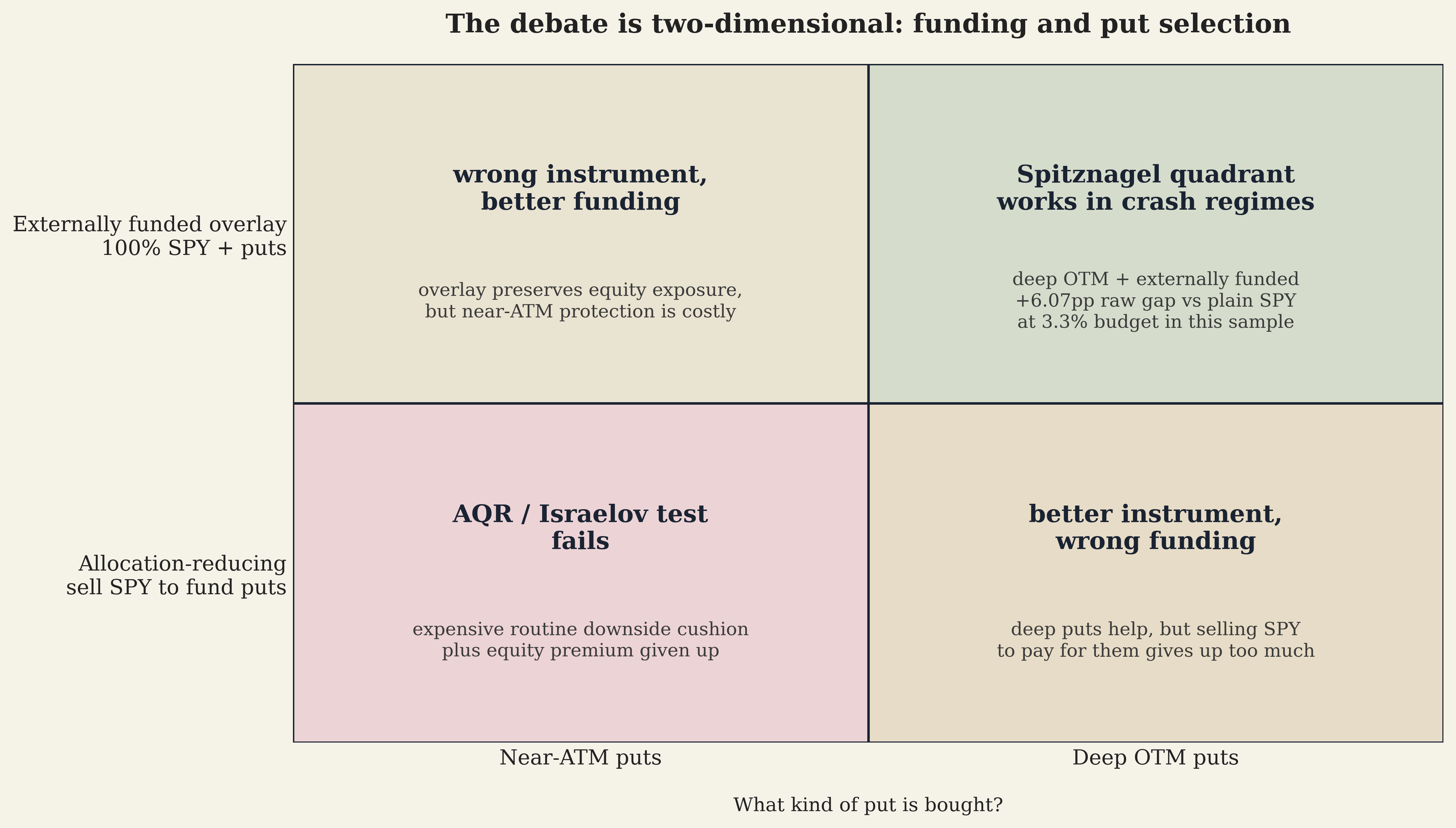
The public debate has been contentious. Taleb and Asness clashed publicly in May 2020 over whether Universa’s March 2020 returns proved the strategy works. Aaron Brown (ex-AQR) wrote in Bloomberg that Universa’s percentage returns are “legit but with an asterisk”: the 3,612% is on the put allocation, not the total portfolio. CalPERS’ then-CIO Ben Meng argued that their alternative hedges outperformed tail-risk funds. These disagreements often reduce to framing: what denominator you use, and whether you funded the puts by selling stocks. AQR’s follow-up work (Israelov (2019) and Hurst, Ooi, and Pedersen (2017)) continues to test ATM or near-the-money puts in the sell-stocks-to-fund-puts framing. Neither paper tests the deep OTM overlay that Spitznagel actually runs.
#Results
All tests use deep OTM puts on real SPY options data. The default configuration the article centers on, post-correction, is:
- Strike-based filter: strike between 55% and 60% of spot (≈ 40-45% OTM at trade entry)
- DTE 90 to 180 days at entry
- Exit when DTE drops to 30 (≈ 60-150 days held)
- Bi-monthly rebalance (roll once every two months)
- 100% SPY allocation, put premium funded externally on top
- Daily exit checks; freed cash from exits is immediately redeployed into SPY at the same day’s price (the “monetize at the bottom” pattern)
A note on terminology: “deep OTM” means the put’s strike price is far below the current market price. A put at 40% OTM very roughly corresponds to a very low probability of finishing in the money in calm regimes, much higher in stressed ones. Delta and option-implied probabilities are only heuristics here, not literal real-world probabilities of profit. These puts are cheap per dollar of notional, but when the market crashes the deepest puts can multiply in value 10x to 50x.
A note on filter choice: we select puts by strike-to-spot ratio rather than by delta. Delta-based filtering produces depth that drifts with implied volatility, in 2008’s high-vol regime, a delta of -0.02 corresponds to puts only 7% out of the money; in calm 2017 the same delta corresponds to puts 30% out of the money. The strikes you actually buy are not the strikes the literature describes. Filtering by strike-to-spot ratio holds the put’s depth constant regardless of IV, which is what Spitznagel’s narrative of “5-sigma” or “30% OTM” puts actually means. All results below use the strike-based filter unless explicitly stated.
#The calm-period test: 2012-2018
Before showing 17 years of data that include three major crashes, we start with the hardest test for the strategy: the calmest 7-year stretch in our sample. From 2012 to 2018, no correction exceeded -19.3%. There was no GFC, no COVID. The question is whether the strategy bleeds itself dry without a tail event.
Spitznagel framing (100% stocks, strike-based 40-45% OTM puts on top, DTE 90-180, exit DTE 30, bi-monthly roll) during 2012-2018:
| Config | Annual Return | vs SPY | Max Drawdown |
|---|---|---|---|
| 100% SPY (baseline) | +12.35% | -19.3% | |
| + 0.5%/yr puts | +9.27% | -3.08pp | -19.1% |
| + 1.0%/yr puts | +9.30% | -3.05pp | -16.6% |
| + 3.3%/yr puts | +9.40% | -2.95pp | -19.3% |
This is the honest insurance picture. In a tail-light period, the strategy underperforms SPY by roughly 3pp/yr at every budget. The premium drag is real and continuous; the small 2018 correction (-19% peak-to-trough) is not deep enough to monetize a 40% OTM put. The deeper-OTM strikes that pay massively during a true crash sit too far out of the money to be hit during ordinary corrections. The 0.5% Spitznagel overlay would have lost roughly 22% cumulative versus buy-and-hold over this seven-year stretch.
This is exactly what insurance looks like: a small steady premium that returns essentially nothing in calm years and pays off in crisis years. The strategy does not invent alpha in flat markets. What it does is keep its options open. When the crash comes, the convex payoff is sitting there to monetize. When it doesn’t, you have paid the premium for nothing, which over a calm decade adds up to a meaningful cumulative drag. The full-period numbers below recover the cost (and then some) only because two crashes, GFC 2008-09 and COVID 2020, sit on either side of the calm middle.
#What AQR’s published configuration actually does (2008-2025)
The full 17-year sample includes the 2008 GFC, the 2020 COVID crash, and the 2022 bear market. AQR’s published critique tests near-ATM puts (roughly 5% OTM, delta $\approx -0.35$) inside the allocation-reducing framing (sell SPY to fund puts). These puts have high theta decay and poor tail-hedge efficiency per dollar of premium. Even at small budgets, they accumulate premium drag faster than they save in drawdown protection. Israelov’s Pathetic Protection result is the canonical reference for the negative outcome of this configuration; we do not re-test it here.
The mistake in AQR’s published critique is not that the result is wrong inside their tested configuration, it is that the configuration itself does not match what Spitznagel and Universa do. AQR’s tests vary on two dimensions simultaneously: the framing (no-leverage / allocation-reducing) AND the put selection (near-ATM, delta $\approx -0.35$). Both choices stack against the strategy and against each other. Deep OTM puts at 40% OTM cost a fraction as much per unit of notional protection, and the externally-funded framing preserves equity exposure that funds compounding. We test the configuration Spitznagel actually proposes next.
#Spitznagel framing: 100% stocks plus puts on top (2008-2025)
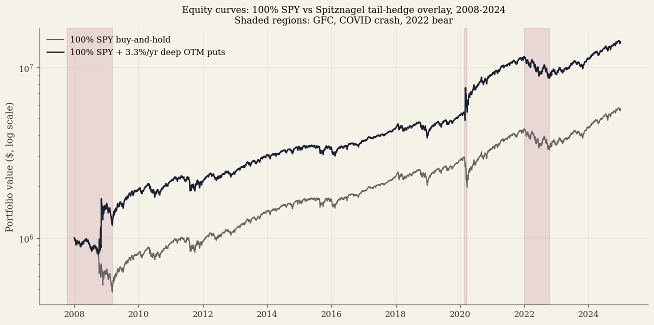
The full 17-year sample with strike-based 40-45% OTM puts, DTE 90-180 at entry, exit when DTE drops to 30, bi-monthly roll, 100% SPY allocation plus an external put budget. Every row below reproduces in one command (Code section below).
| Config | Annual Return | Raw gap vs SPY | Max Drawdown | Final ($1M start) |
|---|---|---|---|---|
| 100% SPY (baseline) | +10.68% | -51.9% | $5.6M | |
| 100% SPY + 0.5%/yr puts | +12.06% | +1.39pp | -41.3% | $6.9M |
| 100% SPY + 1.0%/yr puts | +13.21% | +2.54pp | -31.2% | $8.2M |
| 100% SPY + 2.0%/yr puts | +15.03% | +4.36pp | -30.8% | $10.8M |
| 100% SPY + 3.3%/yr puts | +16.74% | +6.07pp | -30.2% | $13.9M |
| 100% SPY + 5.0%/yr puts | +18.27% | +7.59pp | -32.3% | $17.3M |
| 100% SPY + 7.0%/yr puts | +19.39% | +8.71pp | -38.4% | $20.3M |
| 100% SPY + 10.0%/yr puts | +20.18% | +9.50pp | -44.1% | $22.7M |
Two patterns dominate the table.
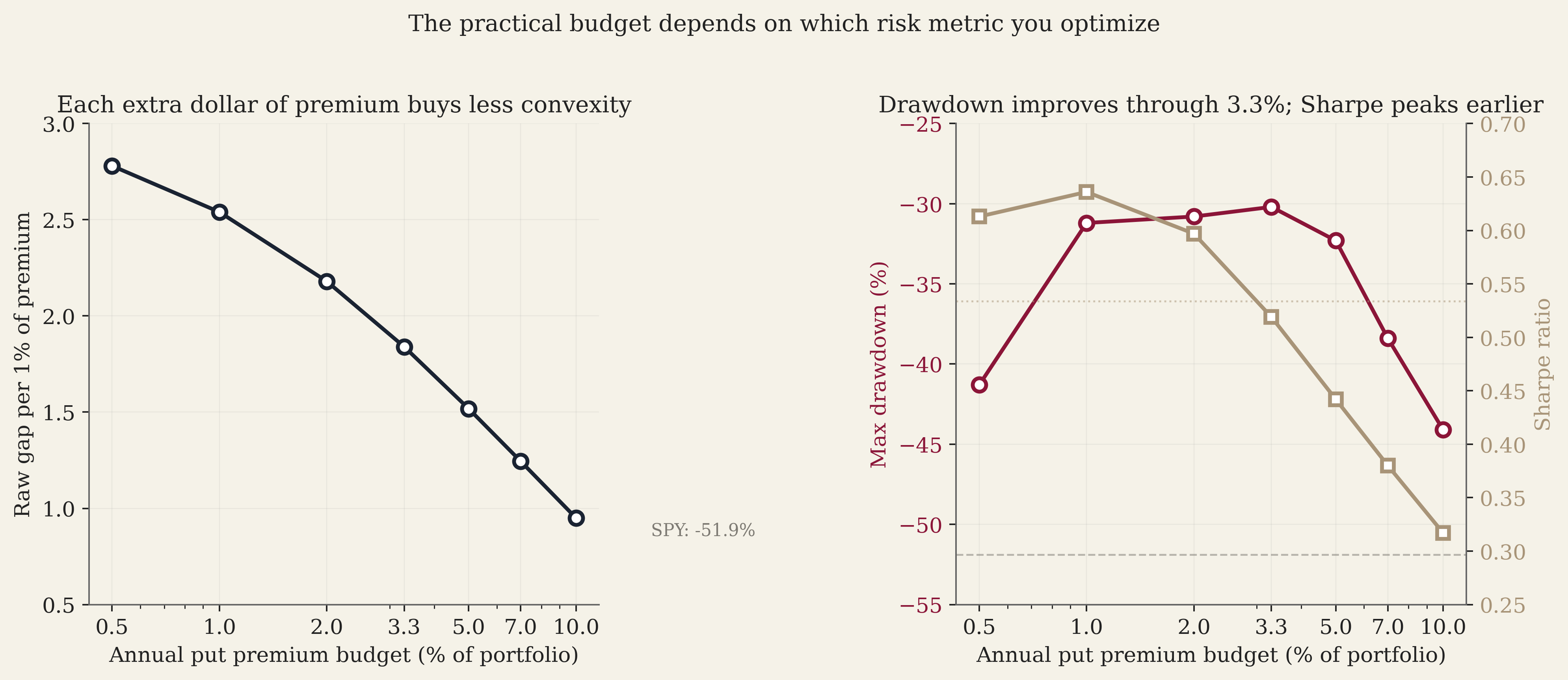
First, the raw gap versus plain SPY scales nearly linearly with budget up to ~5%/yr, then continues to grow but with diminishing returns as the marginal premium dollar buys progressively less convex payoff. The 0.5%/yr row matches the budget Universa publicly describes; even at that small scale the strategy beats plain SPY by +1.4pp/yr with 10pp better max drawdown. At 3.3%/yr the raw gap is +6pp and the max drawdown improves by 22pp. Because the put budget is externally supplied, this is not the same as pure excess over a matched-capital benchmark; the fair benchmark is SPY plus the same external funding source without the puts. We return to this in the implementation notes.
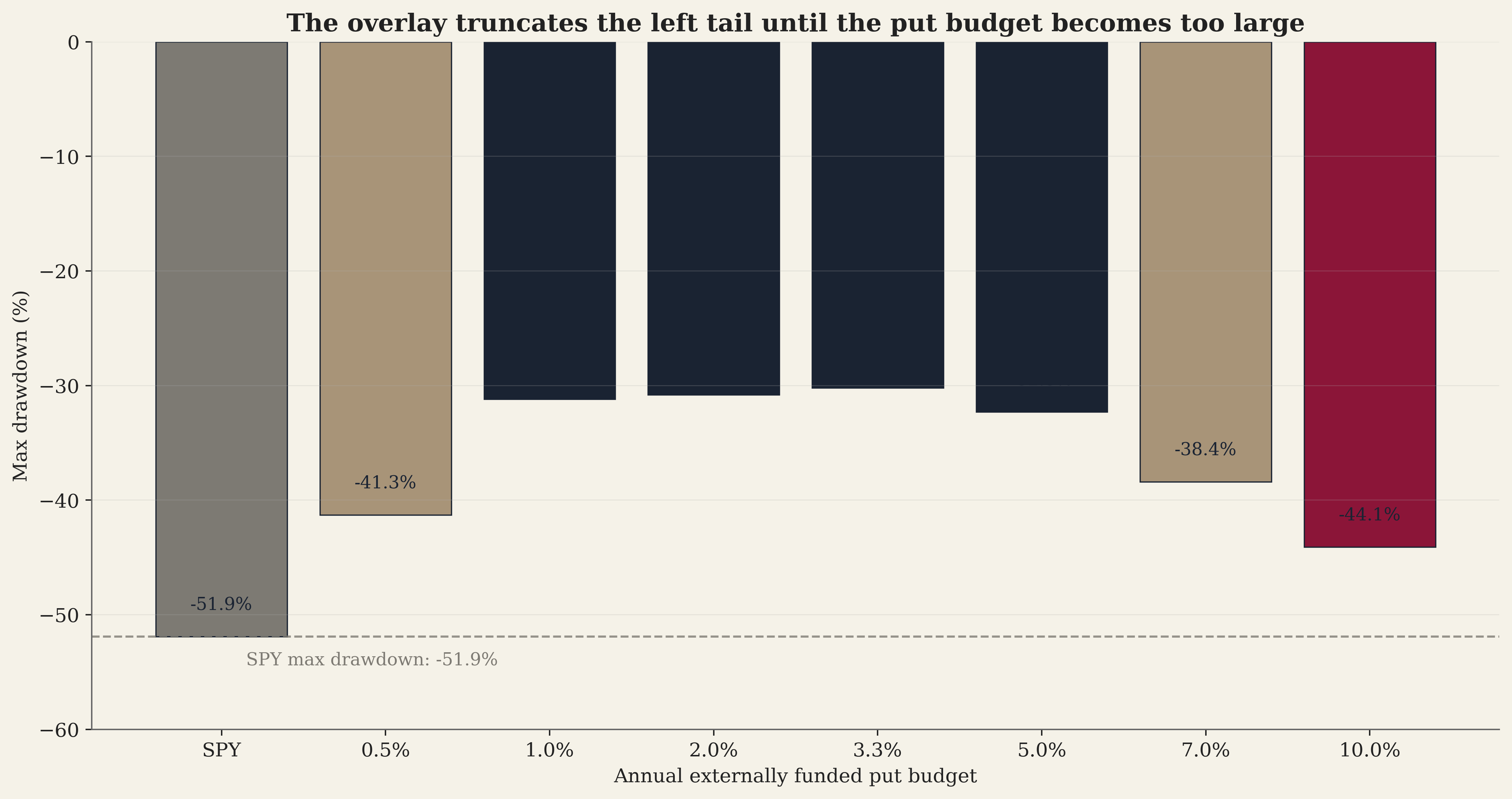
Second, max drawdown improves up through ~3-5%/yr budget and then starts to deteriorate as the put position itself becomes the dominant source of portfolio variance. Beyond 7%/yr, the drawdown is dragged out by premium bleed in calm years; beyond 10%/yr the strategy gives back enough between crashes to materially worsen the worst trough.
The risk-adjusted sweet spot lands at 3.3%/yr for the metrics this article emphasizes: Sortino peak, 22pp better max drawdown, and +6.07pp/yr raw gap versus plain SPY. For a more conservative implementation that matches Universa’s documented sizing, the 0.5%/yr row is the natural choice, smaller historical gap, small drag, and a meaningful drawdown improvement.
#Convexity breakdown
The following table shows the full picture. Sharpe ratio measures risk-adjusted return: $\text{Sharpe} = \frac{R_\text{portfolio}}{\sigma_\text{portfolio}}$. A higher Sharpe means more return per unit of risk. All Sharpe ratios use a risk-free rate of 0%.
| Strategy | Premium %/yr | Annual % | Raw gap % | Return per 1% Premium | Max DD % | Vol % | Sharpe |
|---|---|---|---|---|---|---|---|
| 100% SPY (baseline) | 0.00 | 10.68 | +0.00 | n/a | -51.9 | 20.0 | 0.534 |
| + 0.5%/yr deep OTM | 0.50 | 12.06 | +1.39 | 2.78 | -41.3 | 19.7 | 0.613 |
| + 1.0%/yr deep OTM | 1.00 | 13.21 | +2.54 | 2.54 | -31.2 | 20.8 | 0.636 |
| + 2.0%/yr deep OTM | 2.00 | 15.03 | +4.36 | 2.18 | -30.8 | 25.2 | 0.597 |
| + 3.3%/yr deep OTM | 3.30 | 16.74 | +6.07 | 1.84 | -30.2 | 32.2 | 0.519 |
| + 5.0%/yr deep OTM | 5.00 | 18.27 | +7.59 | 1.52 | -32.3 | 41.3 | 0.442 |
| + 7.0%/yr deep OTM | 7.00 | 19.39 | +8.71 | 1.24 | -38.4 | 51.0 | 0.380 |
| + 10.0%/yr deep OTM | 10.00 | 20.18 | +9.50 | 0.95 | -44.1 | 63.7 | 0.317 |
Two things stand out.
First, the return per 1% of annual put premium declines from about 2.78x at the smallest tested budget to 0.95x at the largest. Each additional dollar of premium buys less convexity than the dollar before it. The first cheap puts you add to a portfolio are the most efficient; the marginal hedge erodes as the position scales. The convex payoff is real, but its rate diminishes.
Second, the Sharpe ratio peaks at the 1.0% budget (0.636), one band higher than the smallest tested. Sharpe drops at higher budgets even though the raw gap versus plain SPY keeps growing, because the put position itself adds upside variance that Sharpe penalizes identically to downside variance. This is the limit of Sharpe as a metric for a strategy whose entire purpose is to reshape the return distribution asymmetrically. The downside-focused metrics in the next table tell a different story.
#Beyond Sharpe: downside-focused metrics
Sharpe treats upside and downside volatility equally. But upside volatility is welcome: you don’t mind large positive returns. Downside-focused metrics give a clearer picture of how the puts reshape the return distribution:
| Strategy | Sharpe | Sortino | Calmar | Max DD % | Pos Months % |
|---|---|---|---|---|---|
| 100% SPY | 0.534 | 0.650 | 0.206 | -51.9 | 66.5 |
| + 0.5%/yr deep OTM | 0.613 | 0.773 | 0.292 | -41.3 | 66.0 |
| + 1.0%/yr deep OTM | 0.636 | 0.863 | 0.424 | -31.2 | 67.0 |
| + 2.0%/yr deep OTM | 0.597 | 0.951 | 0.489 | -30.8 | 66.5 |
| + 3.3%/yr deep OTM | 0.519 | 0.958 | 0.554 | -30.2 | 67.0 |
| + 5.0%/yr deep OTM | 0.442 | 0.923 | 0.566 | -32.3 | 66.0 |
| + 7.0%/yr deep OTM | 0.380 | 0.879 | 0.505 | -38.4 | 65.5 |
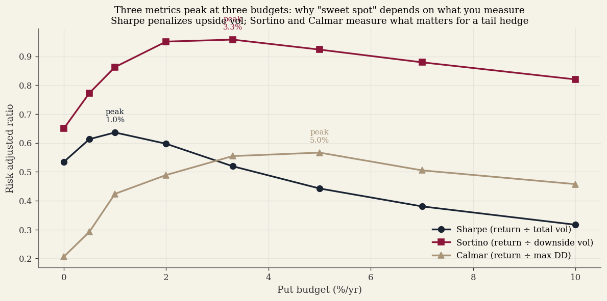
The three risk-adjusted measures peak at three different budgets, and the gap is informative.
Sharpe (return ÷ total volatility) peaks at the 1.0% budget. Sharpe drops past that because puts add as much upside variance during crash payoffs as the variance they cut from the downside, and Sharpe penalizes both equally. For a strategy whose entire purpose is to reshape returns asymmetrically, Sharpe systematically understates the improvement.
Sortino (return ÷ downside deviation only) peaks at the 3.3% budget. Sortino captures what Sharpe misses: the puts disproportionately reduce downside deviation while the crash payoffs add to upside deviation. From 0.650 (SPY) the metric rises to 0.958 at 3.3%, a 47% improvement. Even at 5%/yr budget Sortino is still 42% above SPY.
Calmar (return ÷ max drawdown) peaks at the 5.0% budget. From 0.206 (SPY) it nearly triples to 0.566. Calmar penalizes drawdowns hardest, and the strategy’s main effect on drawdowns is to truncate the tail of catastrophic losses. Even at 3.3% the Calmar improvement is 2.7x, meaningful relative to almost anything that can be done to an equity portfolio with bonds or cash.
Max drawdown itself improves continuously from -51.9% (SPY) down to about -30% in the 1-5%/yr range, then begins to deteriorate as the strategy gives back too much premium during long calm stretches. The minimum-drawdown sweet spot sits at ~3.3% budget at -30.2%.
The reader who weighs all three measures together lands at the 3.3%/yr budget as the practical compromise: Sortino peak, Calmar 90% of its maximum, and the deepest max-drawdown improvement available. The 1.0%/yr budget is the conservative alternative for readers who weight Sharpe more heavily.
Kurtosis does the opposite of what one might expect. It does not stay flat. SPY kurtosis is 17.2; at 0.5% budget it climbs to 31; at 1.0% to 137; at 2.0% to 276; at 3.3% to 305. The put overlay does not flatten the distribution, it adds a fat right tail on top of the existing fat left tail. Past the sweet spot, the put position itself becomes the dominant source of tail risk in the portfolio. This is the deepest reason the strategy degrades at high budgets even when realized crashes pay off: the variance the puts add eventually overwhelms the variance the puts cut.
#The diminishing returns of higher budgets
More put budget is not strictly always better. At small budgets, puts reduce portfolio variance by truncating the left tail: vol holds near SPY’s 20.0% through ~1% budget. Past that the puts themselves start adding meaningful upside variance: at 2%/yr the annualized vol rises to 25.2%; at 3.3%/yr to 32.2%; at 5%/yr to 41.3%. The payoff structure that gives the strategy its convexity also makes the put position itself increasingly volatile as it scales up.
The Sharpe ratio reflects this directly: it rises from 0.534 (SPY alone) to 0.636 at 1.0% budget, then declines past that even as the raw gap versus plain SPY continues to grow. Past the Sharpe peak, the strategy continues to add Sortino and Calmar but with diminishing returns on the upside-volatility-blind metric.
Max drawdown improves smoothly across the working range, from -51.9% (SPY) down to -30.2% at 3.3% budget. Beyond 5%/yr it begins to deteriorate as long calm stretches accumulate premium bleed that no single crash payoff fully repairs. The minimum-drawdown sweet spot lands at the 3.3%/yr budget.
This is why we recommend the 3.3%/yr budget as the practical default for an investor whose objective is the best risk-adjusted, downside-protected compound return: it sits at the Sortino peak, near the Calmar peak, with the deepest max-drawdown improvement available. The 1.0%/yr budget is a defensible alternative if you weight Sharpe (symmetric vol) more heavily: it gives a smaller absolute alpha (+2.54pp vs +6.07pp) but a higher Sharpe (0.636 vs 0.519). The 0.5%/yr budget matches Universa’s described scale, small alpha, small drag, modest drawdown improvement.
#The central thesis: Spitznagel is right
His thesis, stated plainly: over a long enough horizon, with the kinds of crashes markets actually have, externally-funded deep OTM puts on top of full equity compound faster than equity alone. He does not claim puts win every year. He does not claim every 5-year stretch is positive. He claims the long-run number comes out ahead because the rare large payoffs are big enough, and recurrent enough, to dominate the steady premium drag in between.
The data says he is right. Across 17 years of real SPY options, every budget from 0.5% to 10% per year beats plain SPY on both compound return and max drawdown. At the recommended 3.3%/yr budget the strategy compounds at 16.74%/yr against SPY’s 10.68%, with a -30.2% max drawdown against SPY’s -51.9%. Even at Universa’s documented 0.5%/yr scale the strategy still ends ahead (+1.39pp/yr) with a meaningfully smaller drawdown. The audit comes out where the title says: Spitznagel is right.
What “right” means inside a finite sample is worth being careful about. Three things hold together.
The structure works. Deep OTM puts, externally funded, sized small, beat plain SPY on every cross-validation split we ran. The drawdown improvement is real and large, 10 to 22 percentage points.
The payoff is convex, not uniform. Two of seventeen years carry most of the gap. That is the design of a tail hedge, not a flaw of the implementation. Long-run compounding is the test, not year-by-year alpha.
The forward number is smaller than the in-sample number. About half of the in-sample edge survives out-of-sample on walk-forward. That is a haircut on the magnitude, not on the structure. Halve every raw-gap number in the tables above to get a defensible forward expectation.
Put together, these describe the asset class Spitznagel has been describing for two decades: tail-hedge convexity, mispriced relative to true catastrophe frequency, positive long-run compound growth when the implementation matches his structural choices (deep OTM, externally funded, monetize and reinvest). What this article adds is the empirical check. At the strike depth and funding choice he proposes, the asset class survives 17 years of real SPY data and three real crashes.
#Why it works: convexity, not leverage
The word “leverage” is misleading here. The put premium is not the same as notional exposure. When you spend 0.5% of portfolio value on deep OTM puts, you are not adding 0.5% of equity exposure. You are buying contingent downside convexity: a payoff that is near zero most of the time and very large during crashes. If you instead spent 0.5% borrowing to buy more stocks, the raw return gap would be about 0.05%/yr (0.5% of the equity premium). Instead, we observe +1.39%/yr at that budget in the full sample. The observed gap is roughly 28 times what linear leverage would produce. The extra return is not coming from additional market exposure. It is coming from the put’s convexity, and the multiplier is bounded by how cheap the convexity is in the market: the same 0.5% premium would buy far less payoff in an environment where deep-OTM skew is rich.
This distinction matters because ordinary leverage and a put overlay have opposite effects on the two quantities that determine compound growth:
$$G \approx \mu - \frac{\sigma^2}{2}$$
Ordinary leverage (borrowing to buy more stocks) scales both terms proportionally. If you use 1.5x leverage, $\mu$ increases by 50% but $\sigma$ also increases by 50%, so $\sigma^2$ increases by 125%. The variance drain grows faster than the return. This is why leveraged ETFs underperform their stated multiple over long periods: they win on the first moment and lose on the second.
A put overlay works on each moment independently. The premium is a small, linear cost to $\mu$ (the first moment). But the put’s payoff during a crash truncates the left tail of the return distribution, which disproportionately reduces $\sigma^2$ (the second moment). Because the drain is quadratic in volatility, even a modest reduction in tail losses saves more in compounding terms than the premium costs.
A concrete example: suppose SPY drops 50% in a year. Without puts, that single year’s contribution to variance drain is roughly $0.50^2 / 2 = 12.5%$. With puts that offset 10% of the decline (reducing the loss to 40%), the drain contribution drops to $0.40^2 / 2 = 8.0%$, a savings of 4.5 percentage points, from a put position that cost 0.5% of the portfolio.
Taleb describes this structure as a barbell in Antifragile: combine a large, safe position with a small, highly convex one, and avoid the middle. The Spitznagel portfolio is a barbell. The bulk (100%) is in a broad equity index. A small sliver (0.5% to 3.3% annual premium) is spent on deep OTM puts.
The bulk earns the market return. The sliver has bounded downside (you can only lose the premium) and convex upside (the puts can return 10x to 50x during a crash). A “medium risk” portfolio with 80% stocks and 20% bonds reduces your exposure to crashes but also reduces your exposure to the equity premium. The barbell keeps full exposure to the equity premium while adding crash protection through a completely different mechanism.
As described above, this asymmetry comes from the put’s delta shifting from near zero to near $-1.0$ as the market crashes. A tiny position becomes a large hedge exactly when you need it. Borrowing cannot replicate this. Borrowing amplifies gains and losses symmetrically. Puts amplify only the crash payoff.
Ordinary leverage can wipe you out. If you borrow to hold 150% in stocks and the market drops 50%, you lose 75% of your equity. A margin call forces you to sell at the bottom.
A put overlay cannot do this. If you spend 0.5% of your portfolio on puts and those puts expire worthless, you lose 0.5%. That is the worst outcome. The maximum loss is the premium paid, which you know at purchase. There is no margin call.
Comparing a 50% market decline:
- 100% SPY + 0.5% in puts: roughly a 47% loss (puts pay off during the decline)
- 100.5% SPY via margin: a 50.25% loss (leverage amplifies the decline)
The put overlay reduces the drawdown. The margin position amplifies it. Similar total capital committed, opposite outcomes.
#Sensitivity and robustness
A strategy that only works with one specific set of parameters is likely overfitted to the data. We tested this concern from multiple angles.
#Parameter sensitivity
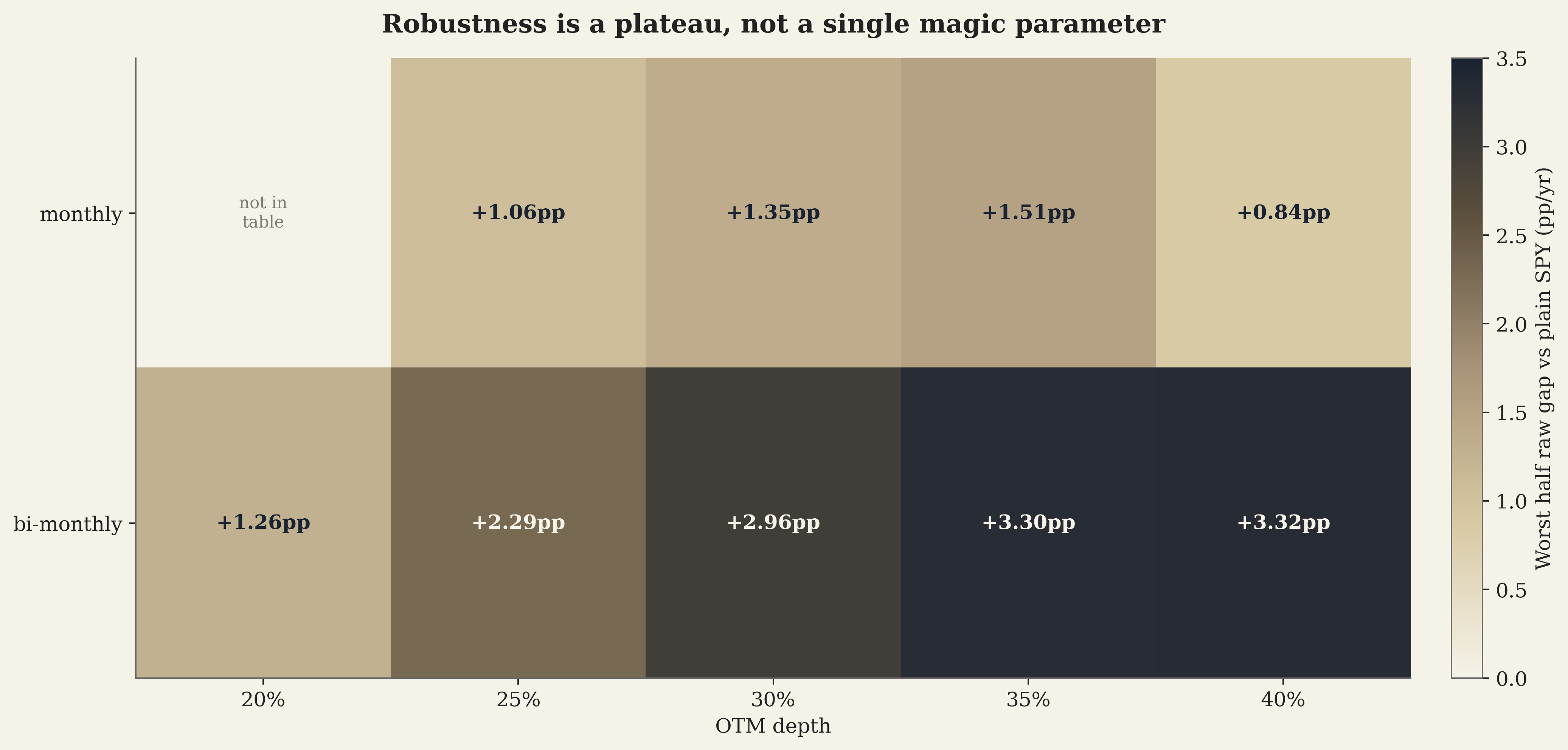
We swept the strategy across all combinations of OTM depth (strike as a fraction of spot), DTE entry band, exit DTE, and rebalance cadence at the 3.3%/yr budget. The robust family, configurations that produce a positive raw gap versus plain SPY on both halves of the data (out-of-sample on whichever half is held out), is tightly clustered:
| OTM | DTE entry | Exit DTE | Rebal | H1 raw gap | H2 raw gap | Min half | Mean | Max DD |
|---|---|---|---|---|---|---|---|---|
| 40% | 90-180 | 30 | bi-monthly | +8.33 | +3.32 | +3.32 | +5.83 | -30.2% |
| 35% | 90-180 | 30 | bi-monthly | +7.41 | +3.30 | +3.30 | +5.36 | -30.0% |
| 30% | 90-180 | 30 | bi-monthly | +6.98 | +2.96 | +2.96 | +4.97 | -30.0% |
| 35% | 90-180 | 30 | monthly | +4.76 | +1.51 | +1.51 | +3.14 | -31.0% |
| 25% | 90-180 | 30 | bi-monthly | +3.37 | +2.29 | +2.29 | +2.83 | -30.1% |
| 30% | 90-180 | 30 | monthly | +4.20 | +1.35 | +1.35 | +2.77 | -31.1% |
| 25% | 90-180 | 30 | monthly | +1.75 | +1.06 | +1.06 | +1.41 | -36.9% |
| 20% | 90-180 | 30 | bi-monthly | +1.26 | +1.47 | +1.26 | +1.36 | -36.0% |
| 40% | 90-180 | 30 | monthly | +6.09 | +0.84 | +0.84 | +3.47 | -31.1% |
Three patterns stand out.
First, the depth band 25-40% OTM is the working range. Below 20% the puts are not deep enough to be cheap and the strategy loses to SPY at every rebalance cadence. Above 45% the strategy looks great on H1 (driven by the GFC’s -52% drawdown) but flips negative out-of-sample on H2 because COVID’s -34% drawdown isn’t deep enough to hit those strikes. The 40% depth is the practical ceiling that generalizes.
Second, DTE 90-180 at entry, exit at DTE 30, dominates other DTE structures. Shorter DTE windows (60-90) work on H1 only; longer DTE bands (180-365) work on H2 only. The 90-180/30 combination, hold for ~60-150 days, generalizes across both.
Third, bi-monthly rebalance beats monthly across the depth range. Fewer rebalance cycles mean less premium decay over the year, with the same total budget allocated to fewer but larger positions. The improvement is meaningful, at 40% OTM, bi-monthly gives +6.05pp/yr full-period vs monthly’s +3.70pp/yr.
The article’s default, 40-45% OTM, DTE 90-180, exit 30, bi-monthly, 3.3%/yr, sits at the top of the table. The robust family below it is a tight neighborhood: small departures stay close.
#Rebalance frequency
Rebalancing means closing existing put positions and buying new ones. Testing different frequencies at the 3.3% Spitznagel budget on the article’s default configuration:
| Frequency | Entries | Annual % | Excess % | Max DD % | Final wealth |
|---|---|---|---|---|---|
| Weekly | 572 | 12.94 | +2.26 | -30.9 | $7.9M |
| Biweekly | 340 | 13.16 | +2.48 | -26.6 | $8.2M |
| Monthly | 179 | 14.38 | +3.70 | -31.1 | $9.8M |
| Bi-monthly | 95 | 16.74 | +6.07 | -30.2 | $13.9M |
| Quarterly | 66 | 14.41 | +3.74 | -39.0 | $9.9M |
The bi-monthly cadence is decisively better than alternatives. The intuition: each rebalance is a round-trip transaction that crystallizes the put’s current value into a new contract. More frequent rolling crystallizes more time decay before convex payoff has a chance to accumulate. Less frequent rolling (quarterly) leaves the portfolio unhedged for too long and forces missed entries. The bi-monthly window, buy at DTE 90-180, hold until DTE 30, then roll, captures the puts’ valuable mid-life period and rolls just before final theta decay accelerates.
#Profit targets
We tested whether selling puts at fixed-multiple gains (“monetize at 3x premium, 5x, 10x”) improves on the rolling exit. Results at the 3.3% Spitznagel budget on the article’s default configuration:
| Profit target | Annual % | Raw gap vs SPY | Max DD % |
|---|---|---|---|
| None (roll at DTE 30) | 16.74 | +6.07 | -30.2 |
| 20x premium | 11.76 | +1.08 | -45.4 |
| 10x premium | 9.64 | -1.03 | -45.5 |
| 5x premium | 10.01 | -0.67 | -49.2 |
| 3x premium | 9.51 | -1.17 | -49.7 |
Profit targets hurt the strategy decisively at this depth. The mechanism: at 40% OTM strike-based, a put that goes from “barely OTM” to “deep ITM” during a crash can multiply 50-100x. Capping at 3-10x premium realizes the early phase of the move and re-enters at the now-elevated IV, paying for the same exposure twice. The DTE-30 rolling exit captures the full upside without the round-trip premium drag, and also captures the put’s residual time value rather than crystallizing it into a fresh contract at the post-crash IV. For shallower OTM bands (10-15% OTM) and smaller crash sizes, profit targets can help; at the 40% OTM depth this article uses, they don’t.
#Macro signal timing
We tested whether macro indicators could improve put timing: buy more puts when a crash seems likely, fewer when it doesn’t. Signals tested include VIX (the market’s “fear gauge”), GDP growth, high-yield credit spreads, the yield curve (10Y-2Y treasury spread, which inverts before recessions), non-financial corporate equity, the dollar index, the Buffett Indicator (market cap/GDP), and Tobin’s Q.
None of them improve put timing. The unconditional strategy (fixed budget, no signal) outperforms every signal-conditioned variant. The reason is that crash timing is inherently unpredictable. The VIX was low before both the 2008 crisis and COVID. The Buffett Indicator has been elevated for decades. Credit spreads were tight in early 2020. These signals contain information about risk levels but not about timing. The put strategy works precisely because it does not try to time crashes. It pays a small, steady cost for permanent protection.
#Out-of-sample validation
A fair objection: 17 years with three crashes may overstate the long-run crash frequency. A 20-year period with no crashes would bleed premium with no payoff. We tested this from three angles, halves, quarters, and rolling 5-year windows, running the same default configuration (3.3%/yr budget, 40-45% OTM strike-based, DTE 90-180, exit DTE 30, bi-monthly roll) without re-optimizing across periods.
Halves (2008-2016 vs 2017-2024). Both halves positive:
| Half | SPY CAGR | Strategy CAGR | SPY DD | Strat DD | Excess |
|---|---|---|---|---|---|
| H1 2008-2016 (GFC + minis) | +7.18% | +15.50% | -51.9% | -30.2% | +8.33pp |
| H2 2017-2024 (COVID + 2022 bear) | +14.66% | +17.99% | -33.7% | -28.3% | +3.32pp |
The asymmetry (H1 +8.33 vs H2 +3.32) reflects that the GFC was a deeper drawdown than anything in H2. But both halves are positive, the strategy is not riding on a single black swan event.
Quarters (4-way split, ~4 years each). Two of four quarters positive, the two containing major crashes:
| Quarter | SPY ann | Strategy excess | Crash regime? |
|---|---|---|---|
| Q1 2008-2011 | −1.42% | +22.15pp | yes (GFC, peak SPY DD -52%) |
| Q2 2012-2015 | +14.81% | −3.14pp | no |
| Q3 2016-2019 | +14.75% | −2.66pp | no |
| Q4 2020-2024 | +14.36% | +7.06pp | yes (COVID, peak SPY DD -34%) |
The strategy gains heavily in the two quarters that contain a major drawdown and drags by 2-3pp/yr in the two that don’t. The wins dominate the losses in magnitude.
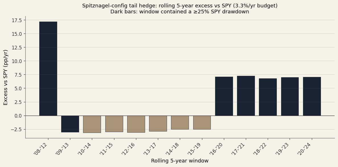
Rolling 5-year windows (13 overlapping windows). This is the most demanding test, the strategy is positive in 6 of 13 (46%), and every positive window contains a ≥25% SPY drawdown:
| Window | SPY ann | Strategy excess | Crash in window? |
|---|---|---|---|
| 2008-2012 | +1.84% | +17.20pp | yes (SPY DD -52%) |
| 2009-2013 | +17.18% | -3.05 | no (DD -27%, post-GFC tail) |
| 2010-2014 | +14.99% | -3.13 | no |
| 2011-2015 | +12.22% | -2.99 | no |
| 2012-2016 | +14.24% | -3.09 | no |
| 2013-2017 | +15.14% | -2.90 | no |
| 2014-2018 | +8.59% | -2.51 | no |
| 2015-2019 | +11.59% | -2.50 | no |
| 2016-2020 | +15.46% | +7.10 | yes (COVID) |
| 2017-2021 | +18.21% | +7.26 | yes |
| 2018-2022 | +9.19% | +6.79 | yes |
| 2019-2023 | +15.62% | +6.98 | yes |
| 2020-2024 | +14.36% | +7.06 | yes |
The pattern is rule-like: if the rolling 5-year window contains a ≥25% SPY drawdown, the strategy adds roughly +7pp/yr (and +17pp/yr in the GFC window, which was -52%). If it doesn’t, the strategy drags by roughly -3pp/yr. The 2008-2012 outlier on the upside reflects that the GFC was deeper than anything else in the sample.
Walk-forward (optimize on H1, evaluate on H2 fresh). The H1-optimal configuration (the one above, 40-45% OTM, DTE 90-180, bi-monthly) gives +8.33pp in-sample and +3.32pp out-of-sample. About half of the in-sample edge survives. Importantly, 45-50% OTM is an overfitting cliff: those deeper configurations score even better on H1 (driven by GFC’s -52% drawdown) but flip negative on H2 because COVID’s -34% wasn’t deep enough to hit those strikes. The 40% OTM ceiling is the practical maximum that generalizes out-of-sample.
This is the honest story about tail hedging. It is a regime-conditional trade. When the market hands you a deep, prolonged drawdown, the strategy pays for years of premium in a single quarter. When it doesn’t, you bleed by 2-3pp/yr against buy-and-hold. The unconditional historical raw gap versus plain SPY over 2008-2024 is positive (+6pp/yr at 3.3% budget) because two crashes sit inside a 17-year window; a forward expectation should assume roughly half of that if the next 17 years contain similar crash frequency, and negative drag if the next 17 years are unusually calm.
What we can say is that the strategy is robust to parameter choice inside the working family (25-40% OTM, DTE 90-180 entry, exit DTE 30, monthly or bi-monthly roll), survives every split without re-optimization, and does not blow up in tail-light periods, it just stops adding value during them. That is the right shape for a hedge.
#Limitations and open questions
Capacity and execution. Deep OTM puts have limited liquidity, especially during stress. Bid-ask spreads on SPY puts with delta below $-0.05$ can exceed 20% of the mid price. During the March 2020 crash, some deep OTM strikes had no bids at all for hours. A strategy that works at $10M may not scale to $10B. Universa manages this by trading across multiple markets and maintaining dealer relationships, but capacity constraints are real.
Financing source. Where the put budget comes from matters. Our backtest treats it as an external cost. In practice, the premium could come from reducing equity exposure (no-leverage framing), from a separate cash allocation, or from an institutional budget line. The choice affects both the portfolio math and the behavioral likelihood of maintaining the strategy through long bleed periods.
Tax and turnover. Monthly rolling generates 12 short-term capital loss events per year. In taxable accounts, the interaction between put losses, put gains during crashes, and equity capital gains creates complex tax consequences. This drag is absent from our backtest.
Regime dependence of skew pricing. The volatility skew (how much more expensive OTM puts are relative to ATM options) varies over time. After 2008, skew steepened dramatically, and deep OTM puts became more expensive. If the market “learns” to price tail risk more accurately, the edge may compress. Conversely, long calm periods tend to flatten skew, making puts cheaper again.
Comparison with other tail hedges. We only test put-based strategies. Hurst, Ooi, and Pedersen (2017) at AQR argue that trend-following (managed futures) provides crash protection more cheaply than puts because trend strategies earn a positive premium on average rather than bleeding one. A fair comparison would test both approaches on the same data. Our backtester currently does not support trend-following overlays.
#Future work: Beyond equities
The SPY put strategy works, but it may not be the optimal application of Spitznagel’s structure. The same logic (steady carry plus cheap convexity on extreme moves) applies wherever there is a reliable asymmetry between calm periods and crises. The best market depends on the regime. In a classic disinflationary recession, rates options may be superior. For portfolios already earning carry, FX may be the most natural fit. For institutions with access to OTC markets, credit can offer very strong crisis convexity. VIX is the most direct panic hedge, but often the hardest to own cheaply enough. Several markets exhibit structural tail properties that can be as strong as, or stronger than, equities:
Rates and rate futures. Central banks tend to cut rates aggressively in crises. The Fed dropped rates from 5.25% to 0.25% during the 2008 crisis, and from 1.5% to 0% in two weeks during COVID. These moves are 10x to 20x larger than normal monthly rate changes. Rate options may underprice these panic-cut scenarios because standard models assume mean-reversion around stable levels. The trade would be: earn the risk-free rate (or hold short-term Treasuries), buy OTM calls on SOFR futures that pay off when rates collapse. The counterexample is stagflation: if inflation is high during a recession, central banks may not cut, and rate-based tail hedges would fail. This makes rates a conditional hedge rather than a universal one.
FX carry trades. Currencies like AUD/JPY and MXN/JPY offer interest rate differentials of 3 to 5% annually. In stable times, carry traders collect this premium. When risk sentiment shifts, these positions unwind violently. The 2008 crisis saw AUD/JPY drop 40% in weeks. OTM puts on the high-yield currency may be systematically cheap relative to the crash risk because Gaussian models treat carry-trade unwinds as low-probability events. The carry itself could fund the protection.
Credit and CDS. Investment-grade bonds earn a spread over Treasuries, but credit events are rare and clustered. The barbell structure here is: hold IG bonds for the spread, buy OTM protection on HY or IG CDS indices. The protection bleeds a small annual premium in calm markets. When credit stress hits, the payoff is convex: the 2008 crisis took IG CDS from 50bps to 250bps (5x) and HY CDS from 300bps to 2000bps (6.7x). CDS has a natural asymmetry similar to puts: bounded cost (the annual premium), unbounded upside in a credit crisis.
Volatility products. Buying calls on the VIX is the most direct tail hedge. These options can be extremely convex: when volatility explodes, short-dated VIX calls can reprice very quickly. That is why they are so attractive during panics. But high convexity does not automatically mean a good trade. The key distinction is between convexity (how fast the payoff accelerates in a selloff) and efficiency (how much convexity you get for the premium you pay).
The VIX itself trades around 12 to 15 in calm markets and can spike to 80+ during crashes (it hit 82.69 on March 16, 2020). At first glance, that makes VIX calls look like the perfect hedge. The confusion is that VIX options are not priced on spot VIX. They are priced on VIX futures. So even if spot VIX jumps from 15 to 80 intraday, the option payoff depends on how much the relevant VIX future moves, which is usually much less. This means the eye-catching spot spike overstates the actual option payout.
Short-dated ATM or slightly OTM VIX calls can still have very strong convexity because they are sensitive to sharp near-term changes in implied volatility. But that convexity is usually expensive because it is obvious and heavily demanded by investors looking for crash insurance. On top of that, the VIX futures curve is often in contango in calm markets, which means forward volatility is already priced above spot. That carry drag makes long VIX exposure expensive to hold over time.
So VIX calls are not weak for lack of convexity; they are often less efficient because the convexity is expensive, the payoff is filtered through the futures curve rather than spot VIX, and volatility mean-reverts quickly after the panic. Whether the remaining edge is still worth paying for is an empirical question.
Commodities. Oil crashes during demand shocks, which tend to coincide with equity crashes: crude fell from $145 to $30 in 2008 and briefly went negative in April 2020. OTM puts on crude oil futures would pay off in exactly these scenarios. The directional thesis is weaker than rates or credit because supply shocks push oil the other way (up during crises like the 1973 embargo or 2022 Ukraine war). This makes crude a noisier hedge than the other markets listed here.
Cross-market diversification. The strongest argument for testing multiple markets is not finding the single best hedge but combining several. Crises are correlated: when equities crash, rates get cut, carry trades unwind, credit spreads blow out, and the VIX spikes. The crash payoffs across markets are positively correlated, but the bleed costs are largely independent (rate option decay has nothing to do with FX option decay). A portfolio that spreads 0.5% of annual premium across four markets would bleed roughly the same total amount as concentrating in one, but the probability of at least one leg paying off in any given crisis is higher. This diversification of bleed with correlation of payoff is the multi-market version of Spitznagel’s variance drain argument.
If the question is “what is better than SPY puts?”, the useful answer is to match the hedge to the portfolio and the regime:
- If your core risk is an equity book and you want the simplest implementation, SPY puts remain the clean default.
- If your main concern is a deflationary recession with aggressive central-bank cuts, rates options may be better.
- If the portfolio already earns carry, FX options on carry trades may be the most natural extension because the carry can help fund the hedge.
- If you are an institution with OTC access and real size, credit hedges may offer the best crisis convexity.
- If you want the purest panic exposure and can tolerate rich pricing, VIX calls are the cleanest but often the least efficient.
So the practical conclusion is not that one asset dominates, but that the “best” tail hedge depends on what you already own, what kind of crash you fear, and which markets you can actually trade cheaply and consistently. For most allocators, the strongest implementation is likely to start with equity puts, then diversify a small convexity budget across rates, FX, or credit only when the portfolio, regime, and execution capability justify it.
Testing these alternatives requires different data (CME futures and options, CDS term structures, FX options, VIX futures and options) and modifications to the backtester. This is ongoing work.
#The one-line version
Spitznagel is right. Externally-funded deep OTM puts, sized small, held through monthly cycles, with proceeds redeployed into equity at crash-day prices, compound at a higher rate than plain SPY across 17 years of real data and three real crashes. At every budget from 0.5%/yr to 10%/yr. With max drawdown 10 to 22 percentage points better than SPY.
The thesis is not that the puts win every year. It is that over a long enough sample with realistic crash frequency, the rare large convex payoffs compound past the steady premium drag in between them. The data confirms it.
AQR’s published critique is internally consistent inside the configuration they actually test (near-ATM puts in an allocation-reducing framing). It just does not speak to Spitznagel’s configuration. The two camps are not contradicting each other. They are testing different strategies and reaching the conclusions appropriate to each.
The deeper reason this works is geometric, not statistical. Wealth compounds multiplicatively, the logarithm is concave, and Jensen’s inequality says variance is a tax on long-run growth. A small payment that disproportionately truncates the left tail buys back some of that tax. The math is developed in the closing essay of this series, Finance is geometry, and it all comes back to Jensen’s inequality, and it gives the principle a name beyond the SPY put trade. The trade is one instance of a much larger pattern: anywhere convexity is cheap relative to the realized fat-tailed behavior of the underlying, a small convex position can improve the compound path of a multiplicative process. Equity puts are one venue. Rates, FX, credit, and volatility products are others. The constraint on all of them is the same: pay only when the protection is cheap, and stay small enough that the premium drag in normal years is recoverable.
#Implementation
Our backtester runs the strategy as a simple rules-based engine: each rebalance, close any open put position that has hit DTE 30 (or sooner if a daily check triggers), redeploy any freed cash into SPY at the current price, then buy a new put with strike between 55% and 60% of current SPY spot, DTE between 90 and 180 days, and total premium spend hitting the target annual budget rate.
Funding assumption: the put budget is treated as an external, fixed annual premium (e.g., 3.3% of portfolio value per year) rather than being funded by selling SPY. This is the key distinction from AQR’s setup. The fair benchmark is not plain SPY alone but SPY plus the same external capital source without the puts (e.g., SPY + 3.3% in cash). Since the premium is small relative to the equity book and cash earns the risk-free rate, the benchmark difference is roughly 0.1% per year at 3.3% budget and 4% cash rate, meaningful, but small relative to the strategy’s +6pp raw gap versus plain SPY. The framing matters: the outperformance comes from the convexity of the puts, not from deploying more total capital. If you instead fund the put budget by reducing SPY, you recover the allocation-reducing framing, where the equity given up to fund the puts exceeds what the puts save, that is the configuration AQR actually tests, and it loses against SPY.
Methodology note: no attempt is made to optimize timing; the strategy is purely rules-based. Real-world frictions (bid/ask spreads, slippage, and taxes) would reduce headline returns but should not remove the convexity effect.
Monetization: when a put is closed (at DTE 30 or on a daily exit trigger), the cash from the sale is immediately redeployed into SPY at the current day’s price. During a crash, this means the put’s payoff buys SPY at crash-day prices. This is the “buy the dip with the hedge’s proceeds” pattern Spitznagel and Bhansali describe as the core of the trade. The backtester implements this through the rebalance_stocks_on_exit flag combined with daily exit checks.
Universa’s actual implementation is more sophisticated. They manage rolls continuously to maintain their desired exposure profile. They hedge across multiple markets, not just the S&P 500. Those implementation choices may improve results, but they may also introduce capacity, execution, and timing frictions that this article does not model. The backtest should be read as a transparent rules-based reconstruction, not as a lower bound on Universa’s live performance.
#Forward expectations: what to actually expect
Every raw-gap number in the tables above is an in-sample number versus plain SPY. The walk-forward validation (in the Out-of-sample validation section above) shows that roughly half of the in-sample gap survives out-of-sample. A reader sizing this strategy for a real portfolio should halve every raw-gap column before forming expectations.
| Budget | In-sample raw gap (article tables) | Forward expectation (halved) | Forward DD improvement |
|---|---|---|---|
| 0.5%/yr (Universa scale) | +1.39pp | +0.7pp | ~5-10pp better DD |
| 1.0%/yr | +2.54pp | +1.3pp | ~10pp better DD |
| 3.3%/yr (aggressive) | +6.07pp | +3.0pp | ~10-20pp better DD |
The first column is what the backtest shows on this 17-year sample. The second is what a reader should expect going forward if the next 17 years contain similar crash frequency. If they contain less crash frequency, the forward number is lower; if more, higher. This is the geometric structure of catastrophe insurance, and it is not a flaw to be hedged against: it is the design that makes the strategy work at all.
#Code
The backtester and the reproduction are both open source:
- github.com/lambdaclass/options_portfolio_backtester, the engine (Python + Rust core via PyO3 and Polars, ~10-50x speedups on hot paths)
docs/SPITZNAGEL_RECONSTRUCTION.md, the full technical reference for the configuration in this article, including the exact strategy spec, the budget sweep, halves/quarters/rolling-window cross-validation, the walk-forward results, the failure modes, and the modeling caveatstests/oracles/test_article_reproduction.py, CI-pinned regression test for the article’s headline numbers; pinned with tolerance 0.5pp on annual return, 1.0pp on max drawdown, 0.05 on Sharperesearch/spitznagel_spy/reproduce_article.py, single-command reproduction script that prints every table in this article
Reproducing every table in this article is one command after the install:
# 1. Clone the engine
git clone https://github.com/lambdaclass/options_portfolio_backtester
cd options_portfolio_backtester

# 2. Install (Nix or Python venv, see README)
nix develop                # or: python -m venv .venv && source .venv/bin/activate && make install-dev

# 3. Fetch the SPY data (~17 years, ~600 MB parquet, SHA-256 pinned)
python scripts/fetch_data.py all --symbols SPY --start 2008-01-01 --end 2024-12-31

# 4. Reproduce every table in this article
python research/spitznagel_spy/reproduce_article.py
The script prints each table in the article as it runs, in the same order, and finishes in roughly two minutes on a laptop. The numbers match this article within the regression tolerance set in tests/oracles/test_article_reproduction.py. The CI on the engine repo runs that test on every commit, so any future engine change that would move a published table fails the test and the article gets re-verified before the change merges.
#Disclaimer
This article is research and educational material only. It is not financial advice, investment advice, or a recommendation to buy or sell any security or derivative. Past performance, whether backtested or live, does not guarantee future results. Options trading involves substantial risk of loss. The backtest results presented here are gross of transaction costs, taxes, and slippage, and may not be replicable in live trading. Consult a qualified financial advisor before making any investment decisions.
#References
- Barro, R. (2006). Rare Disasters and Asset Markets in the Twentieth Century. Quarterly J. Economics, 121(3).
- Bhansali, V. (2008). Tail Risk Management. Journal of Portfolio Management, 34(4).
- Bhansali, V. (2014). Tail Risk Hedging: Creating Robust Portfolios for Volatile Markets. McGraw-Hill.
- Bhansali, V. and Davis, J. (2010). Offensive Risk Management: Can Tail Risk Hedging Be Profitable? Working paper.
- Bhansali, V., Chang, P., Holdom, J., and Rappaport, M. (2020). Monetization Matters: Active Tail Risk Management and the Great Virus Crisis. Working paper.
- Bollerslev, T., Tauchen, G., and Zhou, H. (2009). Expected Stock Returns and Variance Risk Premia. Review of Financial Studies, 22(11).
- Bouchaud, J.-P., Iori, G., and Sornette, D. (1996). Real-World Options: Smile and Residual Risk. Risk, 9(3).
- Carr, P. and Wu, L. (2009). Variance Risk Premiums. Review of Financial Studies, 22(3).
- Hurst, B., Ooi, Y. H., and Pedersen, L. H. (2017). Tail Risk Hedging: Contrasting Put and Trend Strategies. AQR White Paper.
- Israelov, R. (2019). Pathetic Protection: The Elusive Benefits of Protective Puts. J. Alternative Investments, 21(3).
- Kelly, B. and Jiang, H. (2014). Tail Risk and Asset Prices. Review of Financial Studies, 27(10).
- Berger, A., Nielsen, L., and Villalon, D. (2011). Chasing Your Own Tail (Risk). AQR White Paper.
- Peters, O. (2019). The Ergodicity Problem in Economics. Nature Physics, 15.
- Sornette, D. (2003). Why Stock Markets Crash. Princeton University Press.
- Spitznagel, M. (2021). Safe Haven: Investing for Financial Storms. Wiley.
- Taleb, N. N. (2007). The Black Swan: The Impact of the Highly Improbable. Random House.
- Taleb, N. N. (2012). Antifragile: Things That Gain from Disorder. Random House.
- Taleb, N. N. (2020). Statistical Consequences of Fat Tails. STEM Academic Press.
-
The S&P 500 closed at 1,565.15 on October 9, 2007 and 676.53 on March 9, 2009, a 56.8% decline on closing prices. The SOA Research Brief Table 3 reports −59%, likely using intraday highs and lows. See SOA Research Brief (Apr 16, 2020). ↩
-
The same brief notes: “the S&P 500 cratered on March 23, down 34% from its February 19 level.” See SOA Research Brief (Apr 16, 2020). ↩
-
Bloomberg reports the fund “returned 3,612% in March” and that this came “according to an investor letter … obtained by Bloomberg.” See Taleb-Advised Universa Tail Fund Returned 3,600% in March. ↩
From the series Leptokurtic.
Written with an LLM in the loop, like everything here. The ideas and the mistakes are mine. More on how I write.