Ergodicity, Explained: Why the Average Outcome Is Not Your Outcome
A process is ergodic when the average over time equals the average across people. Wealth is not ergodic, and that changes how you should bet, invest and size risk.
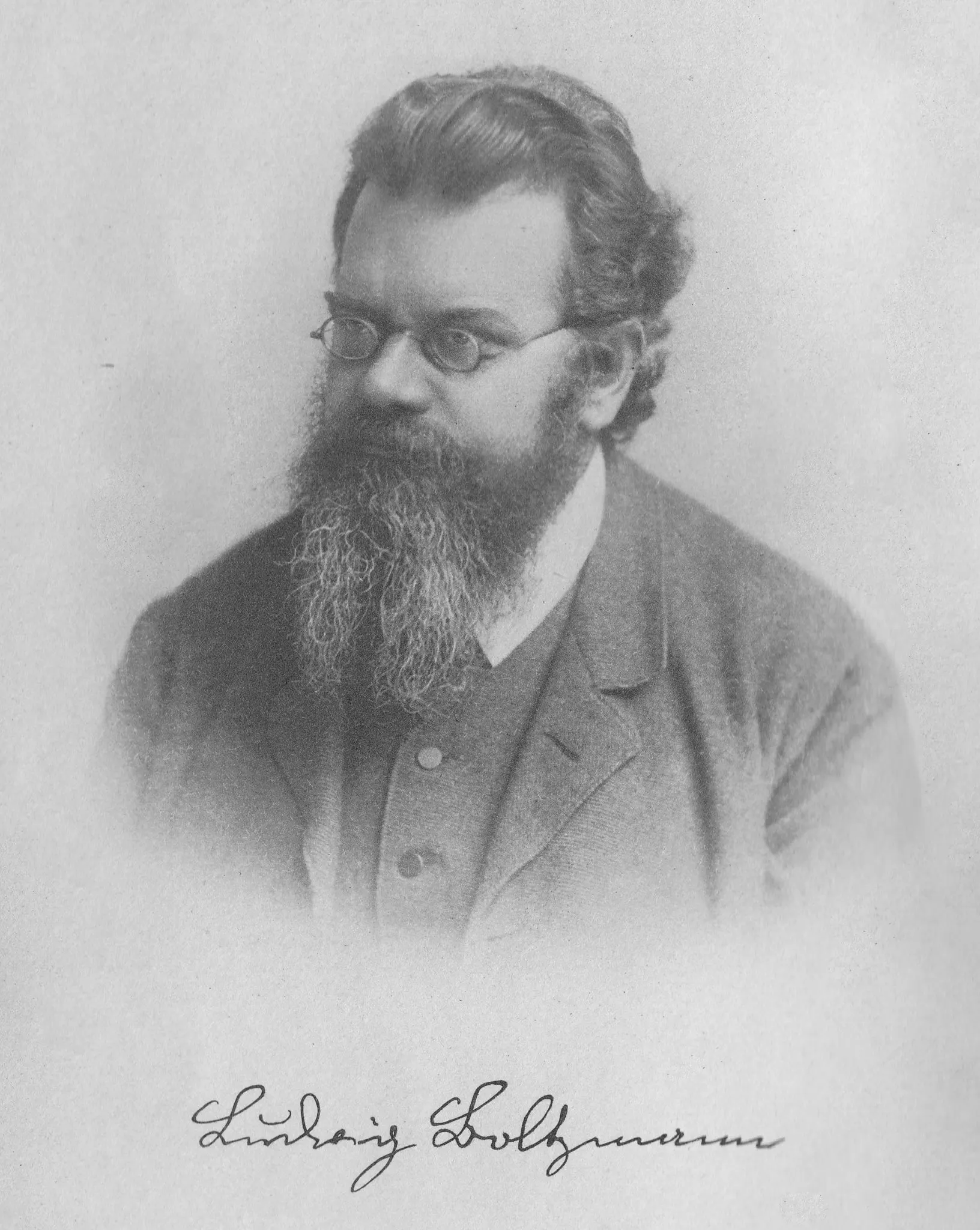
On the image Boltzmann's ergodic hypothesis let physicists replace the history of one molecule with an average over many copies of the gas. That swap is exactly what fails when the thing being averaged is your wealth. Ludwig Boltzmann, the Austrian physicist, in 1902. Photographer unknown, public domain, via Wikimedia Commons.
A process is ergodic when the average over time, for one participant, equals the average across many participants at a single moment. Wealth is not ergodic. The average wealth of a group can grow while almost every person in it gets poorer. That is why the expected value of a bet is the wrong guide for decisions you repeat with the same money.
This is the short version of an idea that runs through most of what I write about finance. The long versions are linked at the end.
#One coin, two answers
Take a coin. Heads, your wealth is multiplied by 1.5. Tails, it is multiplied by 0.6. Is it a good bet?
The textbook answer says yes. The expected outcome of one toss is $0.5 \times 1.5 + 0.5 \times 0.6 = 1.05$, a 5% gain. Give the coin to ten thousand people, let each toss once, and the group as a whole is 5% richer.
Now play it yourself, a hundred times in a row, starting with 100 dollars. Heads and tails each come up about fifty times. Fifty gains of 50% and fifty losses of 40% leave you with
$$\$100 \times 1.5^{50} \times 0.6^{50} = \$100 \times 0.9^{50} \approx \$0.51$$
That is fifty-one cents. Per round, your wealth shrinks by a factor of $\sqrt{1.5 \times 0.6} = \sqrt{0.9} \approx 0.95$, a loss of about 5% each time.
Both numbers are right. The expected wealth after a hundred tosses is about 13,150 dollars, because $1.05^{100} \approx 131$. The median player ends with about fifty cents, and only about 14% of players finish above where they started. The expected value is carried by paths with around 71 heads out of 100, which are so rare that among ten thousand players you would most likely not see a single one. The average is real as arithmetic, and nobody lives it.
The first number is the ensemble average: across people, at one moment. The second is the time average: one person, across many rounds. When the two agree, the process is ergodic and you can use either. Here they point in opposite directions.
#Why they split
The coin multiplies. A 50% gain followed by a 40% loss does not leave you 10% up, it leaves you at $1.5 \times 0.6 = 0.9$, down 10%. Losses hit whatever you have built, and gains have to rebuild from what is left.
Change the coin so it adds instead. Heads you win 50 dollars, tails you lose 40 dollars, no matter how much you have. Now the average across people and the path of one person agree: both gain about 5 dollars a round. Additive bets are ergodic. The trouble starts when outcomes compound, which is the case for savings, portfolios, companies, and most things that grow.
For a multiplicative process, the number that governs one person through time is the average of the logarithm of the growth factor:
$$g = \mathbb{E}[\ln(\text{factor})] = 0.5 \ln 1.5 + 0.5 \ln 0.6 \approx -0.053$$
The ensemble average is the logarithm of the average factor, $\ln 1.05 \approx +0.049$. Because the logarithm bends downward, the first is always below the second whenever outcomes vary. That gap is Jensen’s inequality, and it is the whole reason the averages split.
#Where the word comes from
Ludwig Boltzmann needed a shortcut in the 1870s. To compute the properties of a gas, you would have to follow one molecule for a very long time. He assumed instead that a molecule, given enough time, visits every state the gas allows, so its history looks like a snapshot of many molecules at once. With that assumption, time averages and ensemble averages are interchangeable, and statistical mechanics becomes tractable. That is the ergodic hypothesis.
Economics borrowed the shortcut without the assumption. Expected value, and much of expected utility theory, averages over possible worlds as if the investor could live all of them. In 2019 the physicist Ole Peters published “The ergodicity problem in economics” in Nature Physics, arguing that this is the central mistake: a person lives one path through time, and for wealth that path does not behave like the average across paths.
#See it happen
The simulation below runs 180 paths of a strategy that gains 0.9% in most periods and loses 58% about once every 80 periods. In expectation the average across paths grows about 0.2% per period, while the typical path shrinks about 0.16% per period. Press replay and watch the red and blue lines separate.
Open this simulation in Explore →
The rare crash is what does it. In the average across paths, a 58% loss is one bad event among many good ones, and the paths that missed it pull the average up. On your own path, it takes away more than half of everything the good periods built.
#What to do with it
If you only live the time average, maximize the time average. For bets you repeat with the same money, that means maximizing the expected logarithm of wealth, which is the Kelly criterion.
Go back to the coin. Instead of betting everything each round, bet a fraction $f$ of your wealth. Heads multiplies your wealth by $1 + 0.5f$, tails by $1 - 0.4f$. The growth rate per round is
$$g(f) = 0.5 \ln(1 + 0.5f) + 0.5 \ln(1 - 0.4f)$$
which peaks at $f = 0.25$, with $g \approx +0.62\%$ per round. Betting everything loses about 5% a round for almost everyone. Betting a quarter makes about 0.6% a round for almost everyone, and after a hundred rounds the median player has about 186 dollars instead of fifty cents. Nothing about the coin changed, only how much of your wealth you put on it.
Three practical consequences follow.
Ruin is different from a loss. Zero is an absorbing barrier: once you hit it, you cannot compound back. An average that includes paths where you went broke is averaging over outcomes you will never get to continue from. Taleb’s version is that you should never cross a river that is on average four feet deep.
Variance is a cost. On a single path, volatility lowers the growth rate even when the average return stays the same. For small returns the drag is about half the variance per period. I wrote a separate short piece on volatility drag.
Paying for protection can raise growth. Insurance has negative expected value across policyholders and can still raise the time-average growth of the one who buys it, if it cuts off the losses that do the most damage to compounding. This is the argument behind tail hedging, which I tested on seventeen years of options data in the tail hedge debate.
#Checked in Lean
The central claim is proved in lean-ergodicity, from the strong law of large numbers. If each round multiplies wealth by an independent factor $G$ and $\mathbb{E}[\ln G] < 0$, then wealth goes to zero along almost every path. Nothing in the hypotheses says anything about $\mathbb{E}[G]$, which can be as large as you like.
theorem ae_wealth_tendsto_zero (G : ℕ → Ω → ℝ) (hpos : ∀ i ω, 0 < G i ω)
    (hint : Integrable (fun ω => log (G 0 ω)) μ)
    (hindep : Pairwise (fun i j => IndepFun (G i) (G j) μ))
    (hident : ∀ i, IdentDistrib (G i) (G 0) μ μ)
    (hneg : μ[fun ω => log (G 0 ω)] < 0) :
    ∀ᵐ ω ∂μ, Tendsto (fun n : ℕ => ∏ i ∈ range n, G i ω) atTop (𝓝 0)
The same repository applies this to the coin itself, on a probability space of infinitely many fair flips, and proves that with probability one a player who bets everything ends with nothing. It also proves the coin’s other numbers, Kelly’s fraction of one quarter, and that the two averages differ for every bet that is not a sure thing.
#The limits
Ergodicity economics is not settled. Paul Samuelson spent years arguing against treating Kelly as the one rational rule, and critics of Peters point out that maximizing log wealth is equivalent to a particular choice of utility function, so expected utility theory can already express it. That is a fair point. What the ergodicity framing adds is a reason to choose the logarithm that comes from the dynamics of compounding rather than from taste.
The clean results also depend on clean assumptions: a known coin, repeated independent bets, and no other income. Real returns have fat tails, and estimating the tail is much harder than estimating the average, which is the subject of the Leptokurtic series.
#Further reading
- Finance Is Geometry, and It All Comes Back to Jensen’s Inequality: the long version, from logarithms to Kelly to tail hedging.
- Power Laws, Extremistan, and Non-Ergodicity: what fat tails do to averages.
- Tails and Uncertainty: this simulation and five more about what data can and cannot tell you.
- Ole Peters. (2019). “The ergodicity problem in economics.” Nature Physics 15, 1216 to 1221.
- John L. Kelly Jr. (1956). “A New Interpretation of Information Rate.” Bell System Technical Journal 35(4).
From the series One Path.
Written with an LLM in the loop, like everything here. The ideas and the mistakes are mine. More on how I write.