Chaos, Fractals, and Renormalization

The previous essay built the local picture. Repeated rules can converge to fixed points, and fixed points can organize nearby trajectories into attractors. But the real subject of this series is not only convergence. It is what happens when convergence starts to fail.

The logistic map gives the cleanest path into the failure:

$$x_{n+1}=r x_n(1-x_n).$$

At small parameter values, the map settles. Increase the parameter, and the attracting fixed point loses stability. The system does not become random immediately. It first becomes periodic. Then the period doubles. Then it doubles again. The road to chaos begins as a sequence of broken attractors.

This essay follows that road from bifurcation to chaos, and then from chaos to geometry. The main surprise is that fractals are not decorative pictures attached to chaos after the fact. They are invariant objects produced by repeated stretching, folding, deleting, rescaling, and returning.

#The Minimum Vocabulary

A parameter is a number inside the rule that changes the rule without changing the state variable. In the logistic map:

$$x_{n+1}=r x_n(1-x_n),$$

$x_n$ is the state and $r$ is the parameter. Changing $x_n$ means moving through the system. Changing $r$ means changing the system itself.

A bifurcation is a qualitative change in long-run behavior as a parameter changes. The equation may still make sense, and the old fixed point may still exist algebraically, but its stability can change. That is why existence and stability must be separated.

Chaos means deterministic unpredictability. The rule has no random term, but nearby starting points separate exponentially. The linear-algebra analogy is an eigenvalue larger than one: a small component in an expanding direction gets amplified. In a nonlinear chaotic system, expansion and folding coexist.

A fractal is a set with structure across scales. Often its dimension is not an integer. The word should not mean “complicated picture.” The important fact is scale structure: zooming reveals new detail rather than a smooth tangent line.

Renormalization means changing scale and asking what remains the same. Instead of studying one orbit, you study a transformation on whole systems. A renormalization fixed point is an object that keeps the same form after coarse-graining or rescaling.

#Bifurcations Cascade Into Chaos

Keep increasing the parameter.

The logistic map does not jump straight from order to total disorder. It walks through a very specific cascade:

$$1,2,4,8,16,\ldots$$

The period doubles. Then doubles again. Then doubles again. The parameter intervals between doublings shrink by a universal ratio:

$$\delta \approx 4.669201609\ldots$$

This is Feigenbaum’s constant.

Period doubling is not the only route to chaos. It is the one this essay uses because it gives the cleanest fixed-point story in function space.

The other classical routes are:

1. Quasiperiodic route. A system lives on a torus with two or more incommensurate frequencies, then the torus breaks down. This is associated with Ruelle and Takens.
2. Intermittency route. A system alternates between long quiet phases and irregular bursts. Pomeau and Manneville studied this route; it often produces power-law-distributed waiting times.
3. Crisis route. A chaotic attractor suddenly changes size or disappears when it collides with an unstable set.

So “bifurcations create chaos” is shorthand. More precisely: changing parameters can destroy simple attractors and produce chaotic invariant sets through several mechanisms. Period doubling is the one where the scaling law is easiest to see.

By chaos, I do not mean “random.” A chaotic system is deterministic, but tiny differences in initial conditions grow so fast that long-term prediction becomes impossible in practice.

The usual phrase is sensitive dependence on initial conditions. If two starting points differ by a tiny amount $\epsilon$, after $n$ steps their distance can grow roughly like:

$$\epsilon e^{\lambda n}$$

for some positive number $\lambda$. That $\lambda$ is the Lyapunov exponent. Positive Lyapunov exponent means nearby points separate exponentially.

So chaos is not absence of rule. It is rule applied so repeatedly that information about the initial state gets amplified beyond usefulness.

The logistic map shows this with almost offensive simplicity. For $r=4$:

$$x_{n+1}=4x_n(1-x_n).$$

Two initial conditions that agree for many decimal places can eventually produce unrelated-looking futures. The rule is deterministic. There is no noise term. But the map repeatedly stretches the interval and folds it back. Each iteration reveals another bit of information about the initial condition and then amplifies it into visible difference.

There is even an exact relationship between the fully chaotic logistic map and the tent map. If:

$$x=\sin^2(\pi\theta),$$

then the logistic map at $r=4$ corresponds to doubling the angle:

$$\theta\mapsto 2\theta \pmod 1.$$

That map is the simplest model of chaos. It shifts binary digits. If:

$$\theta=0.b_1b_2b_3\ldots$$

then:

$$2\theta \pmod 1 = 0.b_2b_3b_4\ldots$$

Each iteration discards the first digit and promotes the next digit. A tiny difference far out in the binary expansion eventually moves to the front. This is sensitive dependence in one line.

This is why chaos is connected to information. The initial condition contains infinitely many digits. The dynamics acts like a machine that reads those digits over time. Finite measurement gives you only finitely many digits, so after enough iterations prediction fails.

The shocking part is not that this number appears in the logistic map. The shocking part is that it appears in many unrelated systems. Fluids, electronic circuits, population models, chemical reactions, and one-dimensional maps with a single hump can all approach chaos through the same ratio.

Why?

Because the systems are not just similar in ordinary physical space; they are approaching the same fixed point in function space.

Renormalization is the operation. You rescale the map around its critical point, compose it with itself, and ask what function remains invariant under that transformation. Feigenbaum found a fixed point not of a number, but of an operator acting on functions.

That is the birth of universality.

The deeper statement is that Feigenbaum’s discovery is a renormalization fixed point.

Take a unimodal map, meaning a one-dimensional map with one hump. Near the onset of chaos, look at every second iterate:

$$f^2=f\circ f.$$

Then rescale space so the picture fits back into the same frame. This defines a renormalization operator on maps:

$$\mathcal{R}(f)(x)= -\alpha f(f(-x/\alpha)),$$

where $\alpha$ is the spatial scaling factor. The exact convention varies, but the idea does not: compose the map with itself, zoom back in, and ask what shape remains.

This is the same idea as looking at a coastline from farther away, then rescaling the picture to compare it with the original. The renormalization operator says:

1. compress many small steps into one larger step,
2. rescale the coordinates,
3. compare the new rule with the old rule.

Universality means there is a function $g$ satisfying:

$$\mathcal{R}(g)=g.$$

That is not a fixed point of the original dynamical system. It is a fixed point of an operator acting on dynamical systems. Feigenbaum’s $\delta$ is an eigenvalue of the linearization of $\mathcal{R}$ around $g$. More concretely, if $r_n$ is the parameter value where period $2^n$ first appears, then:

$$\delta=\lim_{n\to\infty}\frac{r_{n-1}-r_{n-2}}{r_n-r_{n-1}}.$$

The constant is universal because the same renormalization fixed point controls the approach to chaos across a whole class of maps. The details wash out. The operator’s fixed point remains.

This is the first moment where the essay should make the reader stop. We began with $x=f(x)$. Now the object satisfying the fixed-point equation is not a number. It is a function. The transformation acts on a space of rules.

The logistic map is the concrete picture behind that abstract sentence. Its bifurcation diagram contains smaller copies of itself. Between chaotic regions there are periodic windows. Inside those windows, period doubling begins again. The same route repeats at smaller scales.

So the logistic map connects three levels at once:

1. state level: points move by $x_{n+1}=rx_n(1-x_n)$,
2. orbit level: fixed points become cycles and cycles double,
3. rule level: the whole family of maps approaches a renormalization fixed point.

Fractality enters because the third level feeds back into the second. The repeated branching of attractors is governed by a self-similar scaling law. Zoom into the diagram and you do not get smoothness. You get more structure.

#Simulation: Feigenbaum Ratios

Numerically locate the first few period-doubling parameters:

$$r_1,r_2,r_3,\ldots$$

Then compute:

$$\frac{r_{n-1}-r_{n-2}}{r_n-r_{n-1}}.$$

These ratios should approach:

$$\delta\approx 4.669.$$

# Approximate known period-doubling parameters for the logistic map.
rs = np.array([
    3.0000000000,
    3.4494897428,
    3.5440903500,
    3.5644072661,
    3.5687594000,
    3.5696916090,
])

ratios = []
for n in range(2, len(rs)):
    ratios.append((rs[n - 1] - rs[n - 2]) / (rs[n] - rs[n - 1]))

print(ratios)

What the reader should see: the cascade is not arbitrary. Its intervals shrink at a universal rate. The fixed point has moved from state space to function space.

The fourth lesson:

Chaos can appear when bifurcations accumulate around a fixed point in function space.

The bridge from bifurcation to chaos is accumulation.

One bifurcation is a structural change. A cascade of bifurcations is a machine for producing arbitrarily fine distinctions in long-run behavior. At period one, the system remembers almost nothing. At period two, it has two phases. At period four, four phases. After many doublings, the number of distinguishable phases becomes too large for finite observation to resolve.

This matters because chaos is often described psychologically as “disorder.” The Feigenbaum route shows the opposite. Chaos is not a failure of determinism. It is determinism iterated through a hierarchy of increasingly fine distinctions.

There is a second bridge here: the object of study moves up one level.

At first we studied points:

$$x\mapsto f(x).$$

Then we studied attractors made of orbits.

Now Feigenbaum asks us to study maps themselves:

$$f\mapsto \mathcal{R}(f).$$

That is a categorical move in spirit, even before category theory enters explicitly. We take the rule that used to act on points and make rules themselves into points of a larger space. The fixed point is no longer a number. It is a universal shape of a function under renormalization.

When the intervals between structural changes shrink geometrically, there is no last simple regime. Order does not disappear because the rule is abandoned. Order dissolves because the rule recursively creates more and more structure than finite measurement can track.

#Chaos Leaves Fractals Behind

Chaotic systems stretch and fold.

Stretch.

Fold.

Stretch.

Fold.

Like kneading dough.

Stretching separates nearby points. Folding keeps the system bounded. Do both forever and a smooth region becomes an infinitely layered object.

This is why strange attractors are fractal. The Lorenz attractor is not just a messy butterfly-shaped picture. It is the geometry left behind by repeated stretching and folding. Points that begin close together separate, loop around, get folded back, and separate again.

Since this essay mostly uses discrete-time maps, the Hénon map is an even better strange-attractor example:

$$x_{n+1}=1-a x_n^2+y_n,$$

$$y_{n+1}=b x_n.$$

For the classical parameters $a=1.4$ and $b=0.3$, the orbit settles onto a thin folded set in the plane. It is not a curve and not an area. It is a strange attractor produced by repeated stretching, folding, and contraction.

A fractal is an object whose detail does not disappear when you zoom in. A smooth curve becomes simpler at small scales. A fractal keeps producing structure. The word often gets abused, but the basic idea is simple: the object has meaningful structure across many scales.

Graphically, the simplest fractal is the Cantor set. Start with the interval $[0,1]$. Remove the middle third. Then remove the middle third of each remaining interval. Then repeat forever.

#Simulation: Cantor Construction

One way to measure this is dimension. A line has dimension 1. A filled square has dimension 2. Some fractals live in between. The Cantor set, for example, has dimension:

$$\frac{\log 2}{\log 3}.$$

Why? At each stage it becomes two copies of itself, each scaled by a factor of $1/3$. If dimension $D$ means “mass scales like length to the $D$,” then:

$$2\left(\frac{1}{3}\right)^D=1,$$

so:

$$D=\frac{\log 2}{\log 3}.$$

Here is the deeper connection back to Banach.

The Cantor set is not just the product of a recursive drawing trick; it is a fixed point of a contraction operator acting on sets.

Define two contractions:

$$S_0(x)=\frac{x}{3},\qquad S_1(x)=\frac{x+2}{3}.$$

Given a compact set $K$, meaning closed and bounded, define the Hutchinson operator:

$$\mathcal{H}(K)=S_0(K)\cup S_1(K).$$

Read this as: take the whole set, make two shrunken copies of it, and union those copies. The input is a shape; the output is the next approximation to the shape.

The Cantor set $C$ satisfies:

$$C=\mathcal{H}(C).$$

That is a fixed-point equation. The difference is that the object is no longer a number. It is a compact set.

The space of compact sets can be given a distance called the Hausdorff metric. It measures how far two shapes are from each other by asking how much one shape must be thickened before it covers the other, and vice versa. Under that metric, $\mathcal{H}$ is a contraction. So Banach’s fixed-point theorem applies again:

repeated contraction produces a unique fixed point.

This is the cleanest possible bridge between the beginning of the essay and fractals. The Cantor set, Sierpiński triangle, and Barnsley fern are fixed points of contractions on spaces of sets. Fractals are not just aesthetically similar to fixed points. Many of them are literally Banach fixed points in a richer space.

#Why roughness is generic

A natural objection: if fractals are just Banach fixed points, why are these fixed points rough rather than smooth? Nothing about contraction sounds jagged, and the fixed points of the first essay were tame.

The answer is a comparison of requirements. A smooth invariant set asks a lot of a map. The set must map into itself, and the map must respect the set’s differentiable structure, carrying tangent directions to tangent directions at every point. That is a strong compatibility condition between the dynamics and the geometry. A fractal invariant set asks for much less: contraction, copying, folding, splitting, and invariance. No tangent structure has to survive.

The dimension equation makes the comparison concrete, because the Hutchinson fixed point is not automatically fractal, and the exceptions are what explain the rule. The two maps $x/2$ and $x/2+1/2$ have the whole interval $[0,1]$ as their fixed point. Four corner maps at contraction ratio $r=1/2$ fill a solid square. Smooth answers happen exactly when the scaled copies tile perfectly, with no gaps and no overlaps. In the equal-ratio dimension equation $N r^D=1$, that perfect tiling is the arithmetic coincidence that makes $D=\log N/\log(1/r)$ come out an integer: two copies at ratio $1/2$, four copies at ratio $1/2$. The formula gives the Hausdorff dimension when the copies do not overlap too much, precisely when they satisfy the open set condition; if the pieces overlap badly, the simple count can fail. Almost any non-overlapping choice of $N$ and $r$ gives a non-integer. The number $D$ is the similarity dimension: it tells you how the amount of detail changes when you zoom. When $D$ is not an integer, the set is too large to be a cloud of points or a smooth curve, but too thin to fill an ordinary area. So rough self-similar sets are not exotic decorations bolted onto dynamics after the fact. They are often the ordinary fixed points of dissipative nonlinear rules, and the smooth cases are the ones that need an explanation.

The Mandelbrot set is another fixed-point object in disguise. For each complex number $c$, iterate:

$$z_{n+1}=z_n^2+c,\qquad z_0=0.$$

The question is whether the orbit stays bounded. The boundary is infinitely detailed because the same iterative question is being asked at every scale.

The link to fixed points is exact, not decorative. The large heart-shaped region, the main cardioid, is precisely the set of $c$ for which $z^2+c$ has an attracting fixed point: a point $z^\star$ with $z^\star=z^{\star 2}+c$ and multiplier $|2z^\star|<1$. That is the same stability criterion $|f’(x^\star)|<1$ from the logistic map, now in the complex plane. The round buds attached to the cardioid are the parameters where an attracting cycle has replaced the attracting fixed point. The Mandelbrot set is a map of where $z^2+c$ has a stable fixed point, then a stable two-cycle, then four, which is period doubling once again.

The logistic bifurcation diagram is fractal for a closely related reason. For each value of $r$, you iterate the same map many times and plot the long-run values of $x_n$. The horizontal axis is the parameter $r$. The vertical axis is the attractor.

At first the diagram has one branch: one attracting fixed point.

Then two branches: a period-two attractor.

Then four.

Then eight.

Then a dense-looking chaotic region.

But inside the chaotic region, order returns in windows. A famous one is the period-three window. Inside that window, the same story happens again: period three becomes period six, then twelve, then twenty-four, then chaos. Zoom further and similar structures reappear.

There is a famous theorem hiding behind that sentence. Li and Yorke proved that “period three implies chaos” for interval maps. Sharkovskii’s theorem is even stronger: the existence of a period-three orbit forces the existence of orbits of every other period. So the period-three window is not just a curiosity in a picture. It is a sign that the map has crossed into a regime where periodic structure of all orders is available.

This is not exactly self-similarity like the ideal Cantor set, where each copy is perfectly scaled. It is asymptotic and organized by universal constants. But the philosophical point is the same: iteration produces structure at many scales, and renormalization explains why those scales are related.

The logistic map therefore gives a direct path from a one-line recurrence to a fractal-looking object:

$$x_{n+1}=rx_n(1-x_n)$$

becomes:

1. fixed point,
2. cycle,
3. bifurcation cascade,
4. chaos,
5. self-similar bifurcation diagram,
6. fractal invariant sets.

This is the reason it deserves so much attention. It is the whole ladder before the ladder becomes abstract.

The stretch-fold mechanism can be made brutally concrete with the tent map:

$$T(x)=1-2|x-\tfrac{1}{2}|.$$

It stretches the unit interval by a factor of two, then folds it back onto itself. The baker’s map does the same thing in two dimensions: stretch a square, cut it, stack it. Repeated forever, the map creates sensitivity to initial conditions because the stretching separates nearby points exponentially.

#Simulation: Stretch And Fold

Iterate the tent map from many nearby starting points.

import numpy as np
import matplotlib.pyplot as plt

def tent(x):
    return 1 - 2 * np.abs(x - 0.5)

xs = np.linspace(0.1, 0.1001, 50)
paths = [xs]

for _ in range(30):
    paths.append(tent(paths[-1]))

paths = np.array(paths)
plt.plot(paths, alpha=0.35)
plt.xlabel("iteration")
plt.ylabel("x")

What the reader should see: points that start almost indistinguishably close separate quickly. Stretching creates sensitivity; folding keeps the values inside the interval; repetition creates fine structure.

That exponential separation is measured by a Lyapunov exponent:

$$\lambda=\lim_{n\to\infty}\frac{1}{n}\log |(f^n)’(x)|.$$

If $\lambda>0$, nearby initial conditions separate on average. Prediction decays exponentially. But folding keeps the motion bounded, so the system does not simply fly apart. It stays in a finite region while continually producing new distinguishable detail.

For the tent map, this is exact. Away from the folding point, the slope has absolute value $2$, so after $n$ iterates the derivative magnitude is roughly $2^n$. Therefore:

$$\lambda=\lim_{n\to\infty}\frac{1}{n}\log(2^n)=\log 2.$$

The fully chaotic logistic map at $r=4$ has the same Lyapunov exponent, $\log 2$, after the change of variables $x=\sin^2(\pi\theta)$. This is a good example of an abstract definition becoming a number you can actually compute.

That is the geometric recipe for a strange attractor:

1. stretch to create sensitivity,
2. fold to keep boundedness,
3. repeat to generate fine structure.

The fractal is the invariant set of that operation.

The fifth lesson:

Fractals are the geometry left behind by repeated stretching and folding.

The bridge from chaos to fractals is bounded instability.

If nearby points separate and nothing folds them back, the system just disperses. If folding happens without stretching, the system just settles. A strange attractor needs both: expansion to create detail, folding to keep the detail in a bounded region.

This is why chaos leaves geometry behind. Sensitive dependence is a statement about trajectories. A fractal attractor is the spatial trace of that sensitivity after infinitely many rounds of stretching and folding. The dynamics says:

$$\text{nearby states separate}.$$

The geometry says:

$$\text{the invariant set has structure at every scale}.$$

Those are two views of the same process. The first view follows points through time. The second view looks at the set that survives after the process has acted forever.

That is why chaotic attractors often have non-integer dimension. They are not curves, because stretching has multiplied their internal detail. They are not areas, because folding and dissipation keep them thinner than a filled region. A fractal is what remains when instability is trapped.

#Why Fractals Are the Default

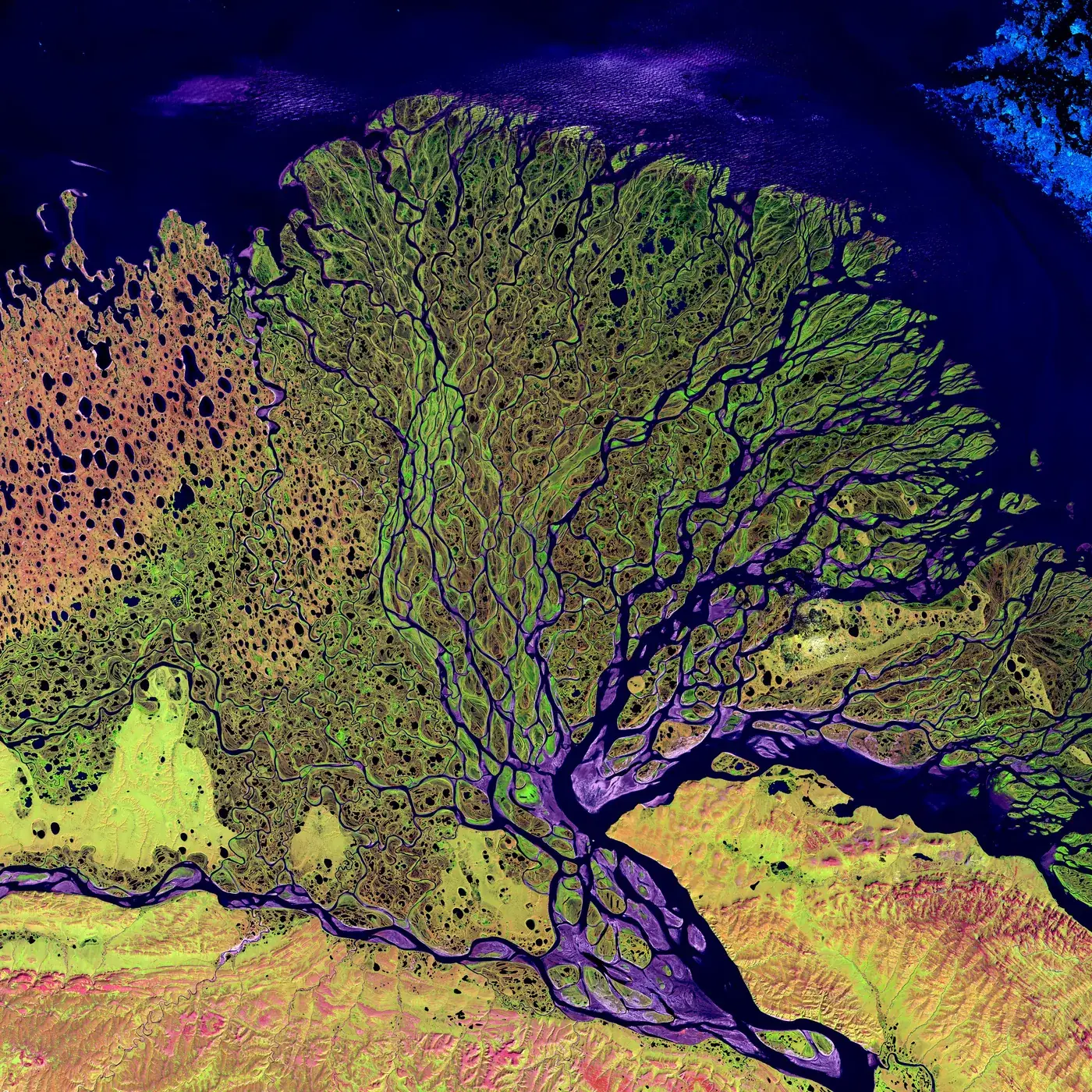
A question has been hiding under this whole essay: why does nature keep producing these objects? River deltas like the one in this essay’s header, lungs, coastlines, mountain ranges, price charts. The standard answer is that growth repeats the same rule at different scales. That is true and explains nothing, because it restates the observation. The better question is why repeated rules leave behind self-similar sets rather than smooth ones.

Start with what self-similarity actually is. If $K=\mathcal{H}(K)$, then $K$ contains scaled copies of itself, and those copies contain scaled copies, without end. Here $\mathcal{H}$ is the set-valued rule from above: take a shape, shrink it, copy it, and put the copies together. Zooming reveals the same structure because the equation says it must. The infinite regress is not a decoration on the answer. It is the content of the fixed-point equation, read geometrically.

The dynamics is what supplies the contractions, and here the essay’s recipe returns. Dissipation alone collapses everything to a point; that is contraction with nothing opposing it. Bounded chaos needs stretch plus fold, and stretch-and-fold applied forever is the Hutchinson picture drawn by the dynamics itself: the strange attractor is the set the kneading leaves invariant. In complex dynamics this becomes sharp. For rational maps of degree at least two, maps of the complex plane built from ratios of polynomials, with $z\mapsto z^2+c$ as the standard family, the boundary between starting points with different long-run fates is the Julia set, and apart from classified exceptional families it is fractal: circles, Chebyshev intervals, and Lattès-type examples are the cases where the roughness is absent or unusually regular. The unit circle, left invariant by $z\mapsto z^2$, is the clean toy exception. In real systems the statement is a strong tendency rather than a law: a double-well gradient flow, a ball rolling with friction on a landscape with two valleys, has two attractors, one valley bottom each, separated by a perfectly smooth basin boundary, the ridge line. The boundary turns fractal when a chaotic saddle lives inside it, an unstable invariant set on which the dynamics is itself chaotic, a tangle that scrambles which side a nearby start will fall to. Forced nonlinear systems arrange that readily. So the lesson is not that every boundary between basins is fractal. It is narrower and stronger: once expansion, folding, and multiple long-run fates coexist, smooth separating surfaces are fragile, and fractal boundaries are the natural outcome.

That is why the same geometry recurs across nature. A branching rule, split into $N$ copies at ratio $r$, is an iterated function system by construction, and lungs and trees run it because its fixed point packs enormous exchange surface into bounded volume. Eroding terrain and growing snowflakes are shaped by their process rates the way $N$ and $r$ set $D$, which is why measured terrain dimensions land between 2 and 3 rather than on either. Price records are self-affine in time, meaning the vertical and horizontal axes rescale differently but the roughness still has no characteristic scale; Mandelbrot saw it in cotton prices in 1963, and the next essay follows that thread into power laws. The cosmic web looks fractal over a finite range of scales and smooths out at the largest. Every one of these is approximate and finite-range, like every empirical scaling in this series. None of them needs a designer of detail. Each needs only a rule with expansion and contraction, applied again.

One boundary should be drawn while the picture is fresh. This is still the iteration engine, not self-reference in the logical sense. A fractal repeats because a geometric rule is iterated on sets. A Gödel sentence, several essays ahead, refers to itself because a formal system can encode its own syntax. Those are different mechanisms. What they share is the fixed-point shape: an object is fed through a transformation and returns as itself, possibly one level up. Later essays use the same abstract shape for syntax, programs, types, life, and markets, and the two engines should not be collapsed into each other.

So the conclusion runs backwards from the intuition. Fractals are not the exotic case; smooth geometry is. Iterate a nonlinear rule with both expanding and contracting directions, the ordinary situation for an interesting dynamical system, and structure at every scale is the default outcome. The real question was never why fractals are everywhere. It is why we expected smoothness, the fine-tuned case, to be the norm.

The invariant summary of this essay is:

$$ \text{stretch}+\text{fold}+\text{repeat}\Rightarrow\text{fractal invariant set}. $$

At the Feigenbaum level the fixed point is no longer a point in state space. It is a function left unchanged by a renormalization operator:

$$ \mathcal{R}(g)=g. $$

At the fractal level the fixed point may be a set left unchanged by an iterated-function-system operator:

$$ \mathcal{H}(K)=K. $$

The point has moved up one level. The next essay moves it up again: from invariant sets to invariant scaling laws and probability tails.

#Further Reading

1. Mitchell Feigenbaum, Quantitative universality for a class of nonlinear transformations (1978). The period-doubling universality paper.
2. Tien-Yien Li and James Yorke, Period three implies chaos (1975). The paper that gave chaos its modern mathematical name in one-dimensional dynamics.
3. Robert Devaney, An Introduction to Chaotic Dynamical Systems. A clear path through symbolic dynamics, chaos, and fractals.
4. Michael Barnsley, Fractals Everywhere. The standard reference for iterated function systems and the Hutchinson operator.
5. Edward Lorenz, Deterministic nonperiodic flow (1963). The continuous-time strange-attractor classic.